Blue light-induced artifacts in glass pipette-based recording electrodes

Recently, I was carrying out whole-cell voltage-clamp and LFP recordings with simultaneous optogenetic activation of a channelrhodopsin using blue light. Whole-cell voltage clamp techniques can record the input currents seen by a neuron (previously on this blog [1], [2]); an LFP records the very small synaptic currents in bulk brain tissue (nicely reviewed by Oscar Herreras); and optogentics with genetically encoded rhodopsins can make neurons fire using light pulses.

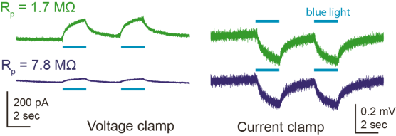
For the LFP recordings, I used the same glass pipette that I had used before for the whole-cell recording of a nearby neuron. In the LFP, I saw a light-evoked response which I first thought was a rhodopsin-evoked synaptic current. However, it turned out that I could make the same observation when positioning the pipette tip in the bath instead of in the tissue, which meant that this was clearly not a synaptic current, but an artifact. When changing the pipette resistance by gently breaking the pipette tip, the light-evoked voltage remained the same, whereas the evoked currents changed proportionally with the pipette resistance Rp, or more generally with the resistance between the two electrodes:
experiment_photovoltaic_effect

I found out that this sort of artifact has been described in the context of tetrode recordings several years ago by Han et al. (2009; supplementary figure 1) and has been sort of explained with the Becquerel effect (here [update 2022: linked website deleted, therefore the link points to an archived version]), which is better known as the photovoltaic effect. According to Han et al., the effect is stronger for blue light and affects the recorded currents on a slow timescale, such that highpass-filtering of the recorded signal, which is used to detect spikes in tetrode recordings, gets rid of this artifact.

In addition, Han et al. state:

We have not seen the artifact with pulled glass micropipettes (such as previously used in Boyden et al., 2005 and Han and Boyden, 2007, or in the mouse recordings described below). Thus, for recordings of local field potentials and other slow signals of importance for neuroscience, hollow glass electrodes may prove useful.

Contrary to this suggestion, my above measurements indicate that using a glass electrode does not or not always get rid of the artifact. To better understand this artifact, I checked whether it was mediated by the chloride silver electrode in the glass pipette or rather by the ground electrode, and found that both contributed more or less equally to the artifact in this experiment. Protection of the electrode by some sort of cover reduced the magnitude of the artifact.

What does this mean for whole-cell or LFP recordings using a glass pipette? For whole-cell recordings, the resistance between the two electrodes is much larger than for the two traces shown in the plots above, typically between 50 and 2000 MΩ. This reduces the artifact-induced current recorded in voltage-clamp to something less than 5 pA for 50 MΩ cells, and much less for neurons with higher membrane resistance. In most cases, this is negligible.

For glass pipette-based LFP recordings or loose seal cell-attached recordings, however, the light-induced voltage change (few hundred μV, as shown above) is of the same magnitude as a strong LFP signal (see for example figure 1 in Friedrich et al., 2004). Therefore, in order to measure a LFP signal in response to blue light-activated rhodopsins, one needs to take into account the artifacts induced by the photovoltaic effect. This can for example be done by measuring the light-evoked voltage change with the glass pipette both in the tissue and in the bath and subtracting the latter measurement from the previous one on a pipette-by-pipette basis.

I would also be curious about other reports (if there are any) on light-induced artifacts with recording electrodes and under which circumstances (if there are any) they might play a non-negligible role.
Posted in Data analysis, electrophysiology, Neuronal activity | Tagged , | 2 Comments

Open access 3D electron microscopy datasets of brains

One of the coolest technical developments in neuroscience during the last decade has been driven by 3D electron microscopy (3D EM). This allowed to cut large junks of small brains (or small junks of big brains) into 8-50 nm thick slices, which are then imaged with nanometer resolution, resulting in 3D stacks of imaged tissue. Here, I want to highlight some of those datasets which are easily accessible in the internet but, at least from my impression, under-used by other researchers.

But also the technical concepts and breakthroughs underlying 3D EM are very interesting. The three main approaches, serial block-face electron microscopy (SBEM), serial section transmission or scanning electron microscopy (ssTEM or ssSEM) and focused ion beam SEM (FIB-SEM) have been very nicely reviewed by a colleague of mine, Benjamin Titze, including some very beautiful and instructive figures (special recommendation for Fig. 4). Of course, this is only a part of the challenge: First, the brain tissue must be stained with heavy metals to be visible for electrons. Second, after data acquisition, human annotators or algorithms have to extract neuronal morphologies or synapse distributions from the huge datasets.

However, I find the raw 3D EM data very interesting by itself. Those datasets are still rare, but many people do not know that some of them are easily accessible to anyone with an internet connection. And it is a true pleasure to have the full screen filled with the overwhelming clutter of neuronal dendrites and to follow them in 3D just by scrolling with the mouse.

Neurodata.io is probably the best place to start. After a simple registration, one can directly access some of those EM datasets in the browser: ndwebtools.neurodata.io/coll_list, or through other tools. Not all of the datasets are of the highest quality (and it is not always easy to judge data quality for a lay person), but most of them offer highly interesting views into the complexity of the brain (scroll wheel for going through the slice, ctrl + scroll wheel for zooming). Here I want to highlight a few of them. They can be accessed by clicking on the neurodata/ndwebtools link above.

The following excerpt by Lee et al. (2016) shows a small zoom-in into the somato-sensory cortex in mouse. A thick dendrite (between the red arrows) is passing vertically through the image. In this ssSEM datasets, synapses look really nice (yellow arrow, with a beautiful vesicle cloud below), but they look even nicer in 3D, so you should have a look at the 3D data yourself.

Lee16_X.png

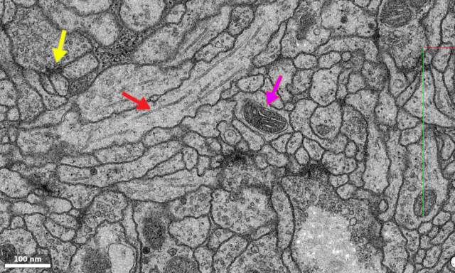
The following picture from a dataset from the Cardona lab shows a small zoom-in of the drosophila brain. (I assume that the scale bar generated for this dataset is a bit off; the 100 nm shown here probably correspond to 500 nm.) The red arrow highlights a filament of the cytoskeleton, probably a microtubule in charge of transport along the dendrite. The pink arrow indicates one of the many mitochondria with its cristae. The yellow arrow indicates a local darkening at the contact site between two neurites, and I have no idea what this is. A gap junction? A strange synapse? A precipitate, i.e., an artifact of the staining procedure?

Cardona.png

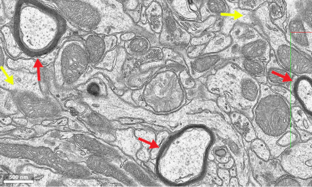
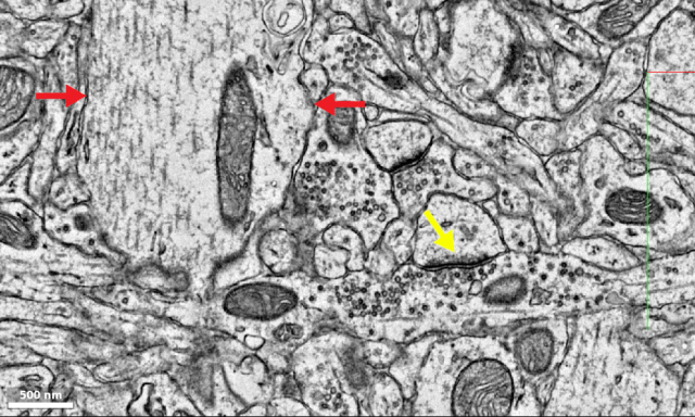
In hippocampus CA1, things look very similar, in a ssTEM dataset used by Bloss et al. (2018). This study focuses on clustering of synapses from single axons. Axons can easily be recognized by their dark and thick myelin sheath (red arrows). If you have a lot of time, you can scroll through the dataset and try to find a node of Ranvier. – As in almost every 3D EM dataset, there are planes or entire regions with low quality staining or low signal to noise imaging or something else that went wrong. Sometimes this is very local, just a blurring of boundaries (yellow arrows) that is difficult to interpret.

Spruston.png

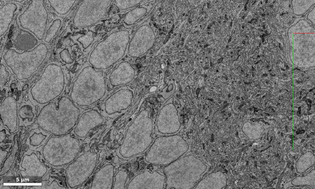
And here is a zoomed-out view of a single plane of a dataset by Wanner et al. (2016) of the olfactory bulb of larval zebrafish. Here, the large roundish shapes are not cross-sections of dendrites, but neuronal somata:

Wanner.png

I just want to encourage people to browse through these datasets. Browsing in 3D is much more interesting than watching these still images. – Or if you are teaching students about neuroscience, why not send them a link such that they can discover neurons themselves by scrolling and zooming through the brains? I haven’t seen many people who were not fascinated when first encountering 3D EM data and who were not overwhelmed by the sheer amount of dendritic arborizations! (And this is a bit funny, if we keep in mind that electron microscopy does not see much of the more complex level of cells, the crowded microenvironment, which is a chaos of competing, interacting, diffusing little protein machines.)

As an alternative to neurodata.io that is accessible even without any registration, a couple of test datasets are available with neuroglancer, a rendering software developed by Google. Check out the dataset from Takemura et al. (2015) by following this link. It is an isotropically resolved dataset (8 nm in x, y and z). You can use the scroll wheel and ctrl to browse through the stack or to zoom in and out. The software includes three EM viewports and an additional rendering of a number of selected neurons.

Another way to explore 3D EM data is to go to eyewire.org, where one can discover 3D EM datasets of neurons (retina, based on Briggman et al., 2011) within the framework of a game – which is fun. Over the last couple of years, the user interface has become very pleasant. The downside compared to the other options is that one cannot discover freely in a big dataset; plus, there is no labeling of the inner organelles or vesicles of the neurons, which is part of the fun for the other datasets.

To understand more details about these EM images, I found it interesting to go through the first chapter of the book Dendrites (“Dendritic structure”), which can accessed almost to its full extent via Google Books.

Full disclosure: my current host lab is working on 3D EM data in zebrafish. My own projects do not involve electron microscopy directly.

Posted in Data analysis, machine learning, Microscopy, Network analysis, zebrafish | Tagged , , , | 1 Comment

How well do CNNs for spike detection generalize to unseen datasets?

Some time ago, Stephan Gerhard and I have used a convolutional neural network (CNN) to detect neuronal spikes from calcium imaging data. (I have mentioned this before, here, here, and on Github.)

This method is covered by the spikefinder paper that was recently published (Berens et al., 2018), based on a competition that featured ground truth for a training and a test dataset. This was a great and useful competition. But there are some important caveats (which are mentioned in the discussion of the main paper). Here, I will discuss one of the caveats.

Continue reading →

Posted in Calcium Imaging, Data analysis, machine learning, Neuronal activity | Tagged , , , , , , | Leave a comment

A list of cognitive biases

There are a handful of cognitive biases that are well-known to most scientists: confirmation bias, the Dunning-Kruger effect, the hindsight bias, the recency effect, the planning fallacy, loss aversion, etc.. Although they should not be taken as universal laws (for example, recently there was some criticism of generalizations of the loss aversion concept), but it is still important to understand which – probably unconscious – biases might shape our behavior, both as humans and as scientists.

I think that some of thoses biases can be useful to think over if one wants to become better at planning (for example of scientific experiments) or better at understanding data and one’s own (biased) interpretation of it. An unusual resource on cognitive biases that I can recommend is the first third of HPMOR, a Harry Potter fanfiction that discusses cognitive biases in the context of an entertaining narrative. And wikipedia offers a more or less comprehensive list of such biases: List of cognitive biases.

I found it very interesting to read through this list. Although some of it is kind of common sense, having a name for a phenomenon can make a difference – similarly, if I know the names of all the trees and plants, wandering through a forest is different from before, because I start to see things not only with my eyes.

Posted in Data analysis, Links | Tagged | 2 Comments

Springtime for two-photon microscopy

Today, the fields and forests around Basel are full of flowers that try to disseminate their pollen. Fixed pollen are, apart from sub-diffraction beads and the convallaria rhizome, one of the most commonly used test/reference samples for fluorescence microscopy. This is both due to their fine, spiky structures and their strong autofluorescence. The scientific study of pollen (and other small things), palynology, provides us with elaborate protocols on how to collect, clean, stain and fix pollen (example 1, example 2) with glycerol jelly between two glass slides.

For two-photon microscopy, these protocols are not ideal since the objectives typically have no correction for glass cover slips between the sample and the objective. Therefore I tested whether it would be possible to look at pollen with a much simpler protocol, using a two-photon microscope. Continue reading →

Posted in Imaging, Microscopy | Tagged , , , | 1 Comment

Layer-wise decorrelation in deep-layered artificial neuronal networks

The most commonly used deep networks are purely feed-forward nets. The input is passed to layers 1, 2, 3, then at some point to the final layer (which can be 10, 100 or even 1000 layers away from the input).  Each of the layers contains neurons that are activated differently by different inputs. Whereas activation patterns in earlier layers might reflect the similarity of the inputs, activation patterns in later layers mirror the similarity of the outputs. For example, a picture of an orange and a picture of a yellowish desert are similar in the input space, but very different with respect to the output of the network. But I want to know what happens in-between. How does the transition look like? And how can this transition be quantified?

To answer this question, I’ve performed a very simple analysis by comparing the activation patterns of each layer for a large set of different inputs. To compare the activations, I simply used the correlation coefficient between activations for each pair of inputs. Continue reading →

Posted in Data analysis, machine learning, Neuronal activity | Tagged , , , , , | Leave a comment

Understanding style transfer

‘Style transfer’ is a method based on deep networks which extracts the style of a painting or picture in order to transfer it to a second picture. For example, the style of a butterfly image (left) is transferred to the picture of a forest (middle; pictures by myself, style transfer with deepart.io):

Stylus_butterfly

Early on I was intrigued by these results: How is it possible to clearly separate ‘style’ and ‘content’ and mix them together as if they were independent channels? The seminal paper by Gatys et al., 2015 (link) referred to a mathematically defined optimization loss which was, however, not really self-explanatory. In this blog post, I will try to convey the intuitive step-by-step understanding that I was missing in the paper myself. Continue reading →

Posted in Data analysis, machine learning | Tagged , , , | Leave a comment

Can two-photon scanning be too fast?

The following back-of-the-envelope calculations do not lead to any useful result, but you might be interested in reading through them if you want to get a better understanding of what happens during two-photon excitation microscopy.

The basic idea of two-photon microscopy is to direct so many photons onto a single confined location in the sample that two photons interact with a fluorophore roughly at the same time, leading to fluorescence. The confinement in time seems to be given by the duration of the laser pulse (ca. 50-500 fs). The confinement in space is in the best case given by the resolution limit (let’s say ca. 0.3 μm in xy and 1 μm in z).

However, since the laser beam is moving around, I wondered whether this may influence the excitation efficiency (spoiler: not really). I thought that his would be the case if the scanning speed in the sample is so high that the fs-pulse is stretched out so much that it spreads over a distance that is greater than the lateral beam size (0.3 μm FWHM).

For normal 8 kHz resonant scanning, the maximum speed (at the center of the FOV) times the temporal pulse width is, assuming a large FOV (1 mm) and a laser pulse that is strongly dispersed through optics and tissue (FWHM = 500 fs):

Δx1 = vmax × Δt = 1 mm × π × 8 kHz × 500 fs = 0.01 nm

This is clearly below the critical limits. Is there anything faster? AOD scanning can run at 100 kHz (reference), although it can not really scan a 1 mm FOV.  TAG lenses are used as scanning devices for two-photon point scanning (reference) and for two-photon light sheet microscopes (reference). They run at up to 1000 kHz sinusoidal. This is performed in the low-resolution direction (z) and usually covers only few hundred microns, but even if it were to cover 1 mm, the spatial spread of the laser pulse would be

Δx1 = 1 mm × π × 1000 kHz × 500 fs = 1 nm

This is already in the range of the size of a typical genetically expressed fluorophor (ca. 2 nm or a bit more for GFP), but clearly less than the resolution limit.

However, even if the infrared pulse was smeared over a couple of micrometers, excitation efficiency would still not be decreased in reality. Why is this so? It can be explained by the requirement that the two photons arriving at the fluorophor have to be absorbed almost ‘simultaneously’. I was unable to find a lot of data on ‘how simultaneous’ this must be, but this interaction window in time seems to be something like Δt < 1 fs (reference). What does this mean? It reduces the true Δx to a fraction of the above results:

Δx2 = 1 mm × π × 1000 kHz × 1 fs = 0.003 nm

Therefore, smearing the physical laser pulses (Δx1) does not really matter. What matters, is the smearing of the temporal interaction window Δt over a spatial distance larger than the resolution limit (Δx2). This, however, would require a line scanning frequency in the GHz range – which will never, ever happen. The scan rate must always be significantly higher than the repetition rate of pulsed excitation. The repetition rate, however,  is limited to <500 MHz due to fluorescence lifetimes of >1-3 ns. Case closed.

Posted in Imaging, Microscopy | Tagged , , , , | 8 Comments

The basis of feature spaces in deep networks

In a new article on Distill, Olah et al. write up a very readable and useful summary of methods to look into the black box of deep networks by feature visualization. I had already spent some time with this topic before (link), but this review pointed me to a couple of interesting aspects that I had not noticed before. In the following, I will write about one aspect of the article in more depth: whether a deep network encodes features rather on a neuronal basis, or rather on a distributed, network basis. Continue reading →

Posted in machine learning, Network analysis, Neuronal activity | Tagged , , , , | 2 Comments

All-optical entirely passive laser scanning with MHz rates

Is it possible to let a laser beam scan over an angle without moving any mechanical parts to deflect the beam? It is. One strategy is to use a very short-pulsed laser beam: A short pulse width means a finite spectral width of the laser (->Heisenberg). A dispersive element like a grating can then be used to automatically diffract the beam into smaller beamlets which in turn can somehow be used to scan or de-scan an object. This technique is called dispersive fourier transformation, although there seem to be different names for only slighly different methods. (I have no experience in this field and am not aware of the current state of the art, but I found this short introductory review useful as a primer.)

Recently, I stumbled over an article that describes a similar scanning technique, but without dispersing the beam spectrally: Multi-MHz laser-scanning single-cell fluorescence microscopy by spatiotemporally encoded virtual source array. First I didn’t believe this could be possible, but apparently it is. In simple words, the authors of the study have designed a device that uses a single laser pulse as an input and outputs several laser pulses, separated in time and with different propagation directions – which is scanning.

Wu et al. from the University of Hong Kong describe their technique in more detail in an earlier paper in Light Science & Applications, and in even more detail in its supplementary information, which I found especially interesting. First, it looked like a Fabri-Pérot interferometer to me, but it is actually completely different and is not even based on wave optics.

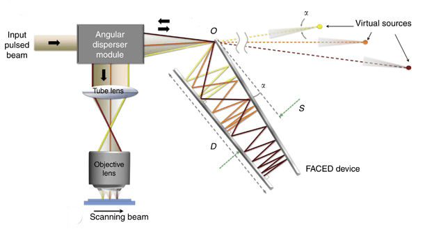
The idea is to shoot an optically converging pulsed beam (e.g. coming from an ultra-fast Ti:Sa laser) into an area that is bounded by two mirrors that are almost parallel, but slightly misaligned by an angle α<1°. The authors call these two misaligned mirrors a ‘FACED device’. Due to the misalignment, the beam will be reflected multiple times, but come back once it hits the surface orthogonally (see e.g. the black light path below). Therefore, the continuous spectrum of incidence angles will be automatically translated into a discrete set of mini-pulses coming out of this device, because either a part of the beam gets reflected 14 times, or 15 times – obviously, there is no such thing as 14.5 reflections, at least in ray optics. This difference of 1 in number of reflections makes the 15-reflection beam spend more time in the device, Δt ≈ 2S/c, with S being the separation of the two mirrors, and c the speed of light.

It took me some time to understand how this works and how these pulselets coming out of the FACED device look like, but I have to admit that I find it really cool. The schematic drawings in the supplementary information, especially figures S1 and S5, are very helpful for understanding what is going on.

ScanSchemeSchematic drawing (adapted) from Wu et al., LS&A (2016) / CC BY 4.0.

As the authors note (without showing any experiments), this approach could be used for multi-photon imaging as well. It is probably true that there are some hidden difficulties and finite size-effects that make an implementation of this scanning technique challenging in practice, but let’s imagine for one minute how this could look like.

Ideally, we want laser pulses that are spaced with a temporal distance of the flourescence lifetime (ca. 3 ns) in order to prevent temporal crosstalk during detection. This would require the two FACED mirrors to be spaced by S = 50 cm, according to the formula mentioned above. Next, we want to resolve, say, 250 points along this fast-scanning axis, which means that the FACED device would need to split the original pulse into 250 delayed pulselets. The input pulsed beam therefore would need to have a pulse repetition rate of ca. 1.3 MHz (which is then also the line scanning frequency), and each of those pulses would need enough power for the whole line scan.

How long would the FACED mirrors need to be? This is difficult to answer, since the answer depends on the divergence angle of the input pulsed beam that hits the FACED device, but I would guess that it needs to be a couple of meters long, given the spacing of the mirrors (50 cm) and the high number of pulselets that are desired (250). (In a more modest scenario, one could envision to split up one pulse of 80 Mhz in only 4 pulselets, thereby achieving multiplexing of additional regular scanning similar to approaches described before.)

However, I would also ask myself whether the created beamlets are not too much dispersed in time, thereby precluding the two-photon effect. And I also wonder how all this behaves like when transitioning from geometric rays to wave optics. Complex things might happen in this regime. – Certainly a lot of work is required to transition this from an optical table to a biologist’s microscope, but I hope that somebody accepts this challenge and maybe, maybe replaces the kHz scanners of typical multi-photon microscopes by a device that achieves MHz scanning in a couple of years.

Posted in Calcium Imaging, Imaging, Microscopy | Tagged , , | 3 Comments