A blog about neurophysiology

Subcellular calcium and voltage imaging of pyramidal neurons in mouse hippocampus

Posted on May 19, 2026 by P.T.R. Rupprecht

Dendrites are the tree-like arborizations of neurons through which they receive input from other neurons. This compartmentalized anatomy has given rise to the idea that individual dendrites process information independently from each other and from the soma. This idea has driven many studies on dendrite function during the last 30 years, mostly in brain slices. But do neurons and dendrites make use of these compartmentalized computations in the intact, living brain?

Recent advances in microscopy and voltage imaging have made it possible to address this question more directly than ever before. Specifially, there has been a recent streak of technically impressive papers on dendritic imaging in the hippocampus of awake mice. In these papers from the labs of Adam Cohen, Attila Losonczy, and Balázs Rózsa, hippocampal pyramidal neurons together with their dendrites are imaged in the behaving mouse, using both calcium and voltage imaging (Gonzalez et al., 2026; Lee et al., 2026; Moore et al., 2025; Wu et al., 2026). Let’s have a closer look!

Paper 1: Two-photon random-access voltage and calcium imaging of CA1 dendrites

Movement-stabilized three-dimensional optical recordings of membrane potential and calcium by Gonzalez, Terada, et al., Neuron, 2026.

Online motion correction for fast dendritic two-photon imaging

Recording both voltage and calcium in 3D is a “holy grail” for dendritic physiology. However, this requires scanning only the dendrites without their surrounding at high speed and repetition rate, making the recording susceptible to artifacts due to brain motion that make such data unusable. To fix this problem, the laser scan pattern needs to be corrected online with millisecond precision to compensate for brain motion. Here, the Rózsa and Losonczy labs developed a new approach that they termed 3D real-time motion correction (3D-RTMC).

Real-time motion correction is highly challenging, and a bright and stable object needs to be used as reference. Earlier work from the lab of Angus Silver injected bright beads for that (Griffiths et al., 2020). Here, the authors took advantage of the single-cell electroporation experts in the Losonczy lab (Gonzalez et al., 2025) and electroporated a cell close to the cell of interest with a fluorescence-expressing plasmid in order have a closeby bright object as a reference for online motion correction. This method allowed them to track the same dendritic branches in a head-fixed mouse running on a treadmill with sub-micron precision using simultaneous voltage and calcium imaging.

Decoupling of calcium vs. voltage with higher dendritic branch order

The authors found that as signals traveled further from the soma, voltage and calcium dynamics became more and more distinct. Proximal dendrite activity mirrored somatic activity, but distal branches showed a progressive decoupling, with branch order, not just distance, determining how well calcium reflected the underlying voltage. A limitation here is that they used the red-shifted jRGECO1a as a calcium indicator (which was necessary so it could be combined with the green voltage sensor ASAP6). jRGECO1a reports calcium changes in a nonlinear way; this nonlinearity is likely to result in missing small dendritic events (Rupprecht et al., 2025).

Local dendritic voltage signals

Interestingly, the authors describe an abundance of local calcium signals in dendrites independent of somatic activity (Figure 2C,K,L; Supplementary Figure 4). However, this important observation is only briefly described and not discussed in depth. For example, Figure 2L shows that dendrites and soma are very likely to be coactive; but if the dendrite is active, the soma is recruited (“s|d”) with a higher probability than the other way around (“d|s”). This is the opposite of what is reported in the paper by (Lee et al., 2026) discussed below and would be worth discussing. – For clarity, the Lee et al. paper came out after the Gonzalez et al. manuscript was published, so the authors had no way to discuss this finding.

Paper 2: Prism-based one-photon voltage imaging of CA1 dendrites

Fast dendritic excitations primarily mediate back-propagation in CA1, by Lee, Park, et al., bioRxiv, 2026.

Prism-based voltage imaging of hippocampal dendrites using one-photon microscopy. Excerpt of Figure 1 from the preprint by Lee et al., under CC BY-NC-ND 4.0 license.

One-photon voltage imaging of individual CA1 neurons

The Cohen lab adapted a previously published design (Redman et al., 2022), using a side-on microprism and kHz-rate voltage imaging with DMD-based structured illumination to record from a large fraction of the entire dendritic tree of CA1 neurons (Lee et al., 2026). This manuscript provides to the best of my knowledge the most comprehensive functional voltage recording of a single neuron in a behaving animal to date.

I’m very impressed by how they combined high-end optics, genetic tools, and very complex data analysis for these experiments in behaving head-fixed mice. From a scientific perspective, the paper is very difficult to summarize because it covers several major questions of neurophysiology in an almost comprehensive manner. And I believe that the choice of the paper title could be improved because it highlights only one aspect of their work.

A note on data analysis

Sometimes, there are Methods sections that are instructive by being rich in interesting details and full of complex processing steps which correct for confounds that you would rarely think of in the beginning: this is one of them. One detail that I found a bit confusing is that they regressed out brain motion (derived from the motion correction algorithm) from the dendritic voltage signals. This is desribed at the bottom of the “Voltage signal extraction” section in Methods. Would this not artificially subtract any dendritic signals related to the movement of the animal? I am a bit skeptic about this methodological detail.

Anti-correlation of apical vs. basal dendrite activity

Lee et al. find that subthreshold voltage is primarily explained by global activity across the entire arbor (~55% of variance), followed by a pattern that they term “see-saw”, where apical and basal dendrites are anticorrelated (~20% of the variance; clearly visible in the movie below). I really like how they collect evidence that this see-saw pattern is most likely determined by laminar-specific inputs in CA1. They do so by comparing the spatial extent of spontaneous activity patterns (large extent) with spatial patterns generated by local dendritic optogenetic depolarization (smaller extent).

Supplementary Movie 3 from the preprint by Lee et al., under CC BY-NC-ND 4.0 license.

Evidence against prominent local voltage events in dendrites

Interestingly, Lee et al. do not find evidence for prominent local voltage events in dendritic compartments, in contrast to the data from the Losonczy/Rósza labs (Gonzalez et al., 2026); and only limited evidence for dendrite-specific place fields, in contrast to a previous calcium imaging study (Moore et al., 2025).

Instead, they find that most “spikes” seen in dendrites originate from back-propagating action potentials (bAPs) in the soma (90%). With this, they identify the soma and not the apical dendrite as primary site of origin for bAPs and complex spikes. In the end, of course, all somatic spikes are caused by the cumulative integration of dendritic inputs. However, this study suggests that the amplification of those signals is primarily a consequence of successful somatic firing and not of amplification in the dendrites, contrasting with existing theories focusing on dendrite-localized amplification (Larkum, 2013; Major et al., 2013; Poirazi and Papoutsi, 2020).

Backpropagation enhanced by local depolarization

The authors also find that apical depolarization enhances bAP propagation into the apical dendrite, which would make bAP propagation specific to sites of prior activity. This finding is not very surprising and confirms earlier work in slices; but it strengthens the idea of bAPs as a learning signal for local dendritic plasticity and is a very important piece of evidence.

Many more biophysical and physiological findings are in the paper, and every paragraph is interesting to read. Highly recommended!

Paper 3: Simultaneous calcium and voltage imaging across the dendritic tree

A dendrite-resolved, in vivo transfer function from spike patterns to Ca2+, by Wu, Lee, et al., bioRxiv, 2026.

One-photon imaging of voltage and calcium in individual neurons

This sister paper from Adam Cohen’s lab also uses prism-based one-photon imaging, recording not only voltage but also calcium events of hippocampal pyramidal cells across a large fraction of the dendritic tree (Wu et al., 2026). To this end, they use a slightly different optical setup, with a spinning disk-based design. They focus on CA2 pyramidal neurons, not primarily for scientific reasons but because expression is much stronger in CA2 for most AAV serotypes (Alexander et al., 2024). Imaging calcium and voltage simultaneously is one of the most interesting experiments for researchers like myself who worked on interpreting calcium imaging data for a long time (Rupprecht et al., 2021, Rupprecht et al., 2025). Achieving such a dual recording across a large fraction of the dendritic tree definitely exceeded my expectations.

A biophysical rule to convert voltage to calcium

Wu et al. find that the mapping from voltage to calcium is remarkably predictable and follows a hierarchical activation pattern. To explain the data, they fit a simple sigmoidal model to the voltage-calcium transfer function. They find that the inflection point of this transfer function (which they term V₀ in their paper) becomes larger for smaller dendritic and especially apical compartments. They argue that this might be a mechanism to avoid noisy dendritic calcium signals due to local depolarizations from synapses. The combination of acquiring such a complex dataset and modeling it in such simple and straightforward terms is quite beautiful.

Similarity to somatic activity decreases with distance from soma for calcium signals and less so for voltage signals. Excerpt from Figure 3 of the preprint by Wu et al., under CC BY-NC-ND 4.0 license.

Further evidence against prominent local events in dendrites

In contrast to previous work based on two-photon imaging data (Gonzalez et al., 2026; Moore et al., 2025), Wu et al. find that localized “dendrite-only” spikes were surprisingly rare. One potential explanation they bring up is that they record from CA2 dendrites, which are know to be less susceptible to plasticity protocols and therefore might not need as prominent local dendritic signals to instruct plasticity as compared to e.g. CA1 neurons. I find this explanation interesting, but I still have the feeling that the dissociation between earlier findings for local events and this evidence against local events is an interesting point of discussion that still needs to be resolved.

Conclusion

First of all: all of these papers are definitely worth reading! I found in particular the two papers from the Cohen lab to be a very interesting resource with many thought-through analyses and in vivo tests of prior brain slice work. The most surprising finding and the largest discrepancy between this work based on one-photon imaging (Lee et al., 2026; Wu et al., 2026) and prior two-photon prism-based work (Gonzalez et al., 2026; Moore et al., 2025; and other work from the Losonczy lab) is the lack of prominent local dendritic activity observed by the work from the Cohen lab.

It is not clear what could explain this discrepancy. Did the approach to regress out brain motion from voltage imaging signals by Lee et al. suppress true local activity? Did the inserted prism cut off connections, resulting in lower activity levels? (This is actually addressed with a control experiment by Lee et al..) Or may two-photon dendritic recordings be more prone to movement artifacts (despite the huge effort to correct for those) and therefore exhibit prominent apparent local activity? It is known that for typical hippocampal windows, the strata radiatum and lacunosum-moleculare, where the apical dendrites reside, exhibit stronger motion artifacts than soma or basal dendrite; in addition, resolution and SNR are lower for apical recordings, all of this contributing to potentially more motion artifacts in apical dendrites. Other reasons that may explain the difference between findings may be the different methods to induce expression, using single-cell electroporation (which adds a lot of plasmids into a single cell and might lead to overexpression) by Gonzalez et al., and AAV-based expression by Wu et al. and Lee et al. (which may have side-effects due to the injected virus particles).

At this point in time, it seems not yet possible to figure out the technical and biological contributions to motion artifacts or the lack thereof in these studies. So I’m really looking forward to seeing these important experiments replicated and consolidated across other labs!

In any case, check out these papers! I barely scratched the surface, and all of them are definitely worth a read.

References

Alexander, G.M., He, B., Leikvoll, A., Jones, S., Wine, R., Kara, P., Martin, N., Dudek, S.M., 2024. Hippocampal CA2 neurons disproportionately express AAV-delivered genetic cargo. https://doi.org/10.1101/2024.11.27.625768

Beaulieu-Laroche, L., Toloza, E.H.S., Brown, N.J., Harnett, M.T., 2019. Widespread and Highly Correlated Somato-dendritic Activity in Cortical Layer 5 Neurons. Neuron 103, 235-241.e4. https://doi.org/10.1016/j.neuron.2019.05.014

Francioni, V., Padamsey, Z., Rochefort, N.L., 2019. High and asymmetric somato-dendritic coupling of V1 layer 5 neurons independent of visual stimulation and locomotion. eLife 8, e49145. https://doi.org/10.7554/eLife.49145

Francioni, V., Tang, V.D., Toloza, E.H.S., Ding, Z., Brown, N.J., Harnett, M.T., 2026. Vectorized instructive signals in cortical dendrites. Nature. https://doi.org/10.1038/s41586-026-10190-7

Gonzalez, K.C., Noguchi, A., Zakka, G., Yong, H.C., Terada, S., Szoboszlay, M., O’Hare, J., Negrean, A., Geiller, T., Polleux, F., Losonczy, A., 2025. Visually guided in vivo single-cell electroporation for monitoring and manipulating mammalian hippocampal neurons. Nat. Protoc. 20, 1468–1484. https://doi.org/10.1038/s41596-024-01099-4

Gonzalez, K.C., Terada, S., Noguchi, A., Zakka, G.N., O’Toole, C., Bilbao, G., Reynolds, L., Jász, A., Kertész, B., Szadai, Z., Shen, A., St-Pierre, F., Polleux, F., Losonczy, A., Rózsa, B., 2026. Movement-stabilized three-dimensional optical recordings of membrane potential changes and calcium dynamics in hippocampal CA1 dendrites. Neuron S0896627326000048. https://doi.org/10.1016/j.neuron.2026.01.004

Griffiths, V.A., Valera, A.M., Lau, J.Y., Roš, H., Younts, T.J., Marin, B., Baragli, C., Coyle, D., Evans, G.J., Konstantinou, G., Koimtzis, T., Nadella, K.M.N.S., Punde, S.A., Kirkby, P.A., Bianco, I.H., Silver, R.A., 2020. Real-time 3D movement correction for two-photon imaging in behaving animals. Nat. Methods 1–8. https://doi.org/10.1038/s41592-020-0851-7

Larkum, M., 2013. A cellular mechanism for cortical associations: an organizing principle for the cerebral cortex. Trends Neurosci. 36, 141–151. https://doi.org/10.1016/j.tins.2012.11.006

Lee, B.H., Park, P., Wu, X., Wong-Campos, J.D., Xu, J., Xiong, M., Qi, Y., Huang, Y.-C., Itkis, D.G., Plutkis, S.E., Lavis, L.D., Cohen, A.E., 2026. Fast dendritic excitations primarily mediate back-propagation in CA1 pyramidal neurons during behavior. https://doi.org/10.64898/2026.01.03.696606

Major, G., Larkum, M.E., Schiller, J., 2013. Active Properties of Neocortical Pyramidal Neuron Dendrites. Annu. Rev. Neurosci. 36, 1–24. https://doi.org/10.1146/annurev-neuro-062111-150343

Moore, J.J., Rashid, S.K., Bicker, E., Johnson, C.D., Codrington, N., Chklovskii, D.B., Basu, J., 2025. Sub-cellular population imaging tools reveal stable apical dendrites in hippocampal area CA3. Nat. Commun. 16, 1119. https://doi.org/10.1038/s41467-025-56289-9

Poirazi, P., Papoutsi, A., 2020. Illuminating dendritic function with computational models. Nat. Rev. Neurosci. 21, 303–321. https://doi.org/10.1038/s41583-020-0301-7

Redman, W.T., Wolcott, N.S., Montelisciani, L., Luna, G., Marks, T.D., Sit, K.K., Yu, C.-H., Smith, S., Goard, M.J., 2022. Long-term transverse imaging of the hippocampus with glass microperiscopes. eLife 11, e75391. https://doi.org/10.7554/eLife.75391

Rupprecht, P., Carta, S., Hoffmann, A., Echizen, M., Blot, A., Kwan, A.C., Dan, Y., Hofer, S.B., Kitamura, K., Helmchen, F., Friedrich, R.W., 2021. A database and deep learning toolbox for noise-optimized, generalized spike inference from calcium imaging. Nat. Neurosci. 24, 1324–1337. https://doi.org/10.1038/s41593-021-00895-5

Rupprecht, P., Rózsa, M., Fang, X., Svoboda, K., Helmchen, F., 2025. Spike inference from calcium imaging data acquired with GCaMP8 indicators. https://doi.org/10.1101/2025.03.03.641129

Wu, X., Lee, B.H., Park, P., Wong-Campos, J.D., Xu, J., Plutkis, S.E., Lavis, L.D., Cohen, A.E., 2026. A dendrite-resolved, in vivo transfer function from spike patterns to dendritic Ca²⁺. https://doi.org/10.64898/2026.01.18.700189

Posted in Calcium Imaging, Data analysis, hippocampus, Imaging, Microscopy, Neuronal activity, neuroscience, Reviews | Tagged Calcium Imaging, Data analysis, Microscopy, Scanning | Leave a comment

CascadeTorch: a PyTorch version of Cascade for spike inference

Posted on February 17, 2026 by P.T.R. Rupprecht

I’m glad to share a PyTorch-based implementation of spike inference from calcium imaging data: CascadeTorch, now available on GitHub.

The original Cascade repository remains fully supported. This post explains why I re-implemented Cascade in Torch, and what this means for users.

What is Cascade?

Cascade is a deep learning-based method for inferring neuronal spike rates from calcium imaging signals (ΔF/F traces). It uses convolutional neural networks trained on a large ground-truth database of simultaneous electrophysiology and calcium recordings. The original publication in 2021 was trained on a broad range of datasets; more recent versions were trained on mouse spinal cord data and, most recently, on variants of the new sensor GCaMP8.

Cascade was originally implemented using TensorFlow/Keras because I this framework showed the highest promise back in 2019/2020. Since then, Cascade has been widely used for spike inference across imaging conditions by many labs.

Why switch to PyTorch?

Since 2021, when we published Cascade, the machine learning community has largely shifted toward other frameworks such as PyTorch or JAX in recent years. An example of this shift in the neuroscience community is DeepLabCut, which recently transitioned from TensorFlow to PyTorch as its primary backend. Installing PyTorch and TensorFlow in parallel is sometimes tricky and can create dependency conflicts of package or GPU driver versions.

What is CascadeTorch?

CascadeTorch is a 1:1 reimplementation of Cascade in PyTorch. That means, the network architecture is identical to the original TensorFlow version, and original pretrained models are simply converted to PyTorch by copying the weights.

Therefore, if you run the same input ΔF/F trace through a TensorFlow model and its converted PyTorch equivalent, you obtain the same spike rate prediction.

Compatibility and support

The original TensorFlow-based Cascade will be fully supported also in the future, and pretrained models are available in both formats. However, if you are starting a new project, I recommend using CascadeTorch. The switch is very straightforward. Simon Ball, who performed some initial tests with CascadeTorch, reported that he’s “getting the same results, and with no changes other than pointing the module import to your forked repository”. Please check out CascadeTorch directly on GitHub:

https://github.com/PTRRupprecht/CascadeTorch

If you have any feedback, please reach out by opening an issue on GitHub or by writing to cascade+p.t.r.rupprecht@gmail.com!

Posted in Calcium Imaging, Data analysis, electrophysiology, Imaging, Microscopy, Neuronal activity, neuroscience | Tagged artificial-intelligence, Calcium Imaging, Data analysis, deep learning, electrophysiology, machine learning, Microscopy, technology | Leave a comment

A clearing method for large human FFPE tissue blocks

Posted on February 8, 2026 by P.T.R. Rupprecht

During the lockdown in 2020, I was forced to stop my own experiments in the lab. This is when I turned to computational and analysis side-projects that since then have become quite central to my own work and approach to science. It was then that I teamed up with Anna Maria Reuss, then PhD student in the lab of Adriano Aguzzi, to work on the analysis of her massive 3D light-sheet imaging data from cleared brains.

Anna Maria developed a method that enables the use of large archival human tissue – non-perfused, and embedded in FFPE for more than ten years -, making it transparent, compatible with antibody labeling, and therefore suitable for imaging at large scale and micrometer resolution.

When you consider the sheer number of such FFPE samples stored in diagnostic archives worldwide, it is clear how powerful this approach is, and how many new lines of research it could enable. Here’s a link to the updated preprint: aDISCO: A clearing method to enable 3D microscopy of large archival paraffin-embedded human tissue blocks.

I’d like to take the opportunity to share this brief movie of a small excerpt of a cleared human brain (dopaminergic neurons in the substantia nigra) that we include in this most recent version of the manuscript to showcase how fine dendrites are resolved:

Dopaminergic neurons in the substantia nigra, a small excerpt from a human brain sample cleared with the aDISCO protocol and imaged with the mesoSPIM light-sheet microscope. Supplementary Movie 2 of Reuss et al., 2026, under CC BY-NC 4.0 license.

Posted in Data analysis, Imaging, Microscopy, neuroscience | Tagged Dopamin, FFPE, Human brain, Light-sheet microscopy, Microscopy, Neuropathology, Pathology, Substantia nigra | Leave a comment

Hippocampal neuron and astrocyte responses to noradrenaline and natural arousal

Posted on February 5, 2026 by P.T.R. Rupprecht

Over the past few years, I worked with Sian Duss, a very skilled and talented PhD student in the lab of Johannes Bohacek, to dissect the role of noradrenaline release in the hippocampus. I’m very excited that the manuscript describing this work is now online as a preprint: Locus coeruleus noradrenaline elicits response profiles distinct from natural arousal in hippocampal neurons and astrocytes.

We used two-photon imaging of interneurons, astrocytes, and pyramidal cells in head-fixed mice, while optogenetically stimulating the primary source of noradrenaline, the locus coeruleus (LC). In addition, we used fiber photometry to calibrate our LC stimulation protocol and to compare optogenetically evoked noradrenaline release with that observed during behavioral paradigms.

For the main findings, please check out the manuscript itself. In this blog post, I’d like to highlight a few results that I personally find fascinating but that are less central in the paper.

1. Astrocytes are much more sensitive to noradrenaline than neurons

Based on our two-photon calcium imaging data, pyramidal neurons and interneurons show little or no response to weaker LC stimulation and respond robustly only to strong stimulation. Astrocytes, in contrast, are highly sensitive and respond even to the lowest detectable increases in LC activity. This positions astrocytes ideally to mediate noradrenergic effects in hippocampal circuits. I find it great to have this very direct comparison across all three cell types – pyramidal cells, interneurons, and astrocytes – using the same experimental approach for each cell type.

Astrocytes are activated both by strong (20 Hz) and intermediate (5 Hz) stimulation of locus coerueleus. A subset of interneurons is activated for strong stimulation (20 Hz), but activation is detectable for weaker stimulation (5 Hz). Adapted from Figure 2 of Duss et al., 2026, under CC BY-NC 4.0 license.

2. Interneurons responsive to noradrenaline are located close to the stratum radiatum

Previous studies have already described that specific functionally defined interneurons are located in specific laminae or sub-laminae of hippocampus (e.g., Geiller et al., 2020). Here, we found that interneurons responding to noradrenaline release upon optogenetic LC stimulation are preferentially located near the pyramidal cell layer, close to the stratum radiatum.

A subset of interneurons is activated by LC stimulation (black traces; Group 1). They are preferentially located in specific laminar positions (bottom right, black density distribution), close to the *stratum radiatum*. Adapted from Figure 5 of Duss et al., 2026, under CC BY-NC 4.0 license.

3. Not all astrocytes are equal

We found that some astrocytes are much more sensitive than others when responding to locus coeruleus activation. These differences were consistent across repeated stimulations and across days. This adds evidence, from a functional perspective, that astrocytes are not a homogeneous population, even within the same hippocampal region.

A functionally defined diversity of astrocytes. Some astrocytes respond at low noradrenaline levels (orange examples), others only at intermediate levels (red), again others only at high levels of noradrenaline release. Adapted from Figure 3 of Duss et al., 2026, under CC BY-NC 4.0 license.

For many more details on the cellular responses to locus coeruleus stimulation, and how these compare to response profiles during natural arousal, check out the preprint. Happy to hear thoughts or questions about the work!

Posted in Astrocytes, Calcium Imaging, hippocampus, Imaging, Locus coeruleus, neuroscience | Tagged Astrocytes, Calcium Imaging, hippocampus, Interneurons, Locus coeruleus, Microscopy, neuroscience, science | 2 Comments

Annual report of my intuition about the brain (2025, part III)

Posted on January 3, 2026 by P.T.R. Rupprecht

How does the brain work, and how can we understand it? To approach this big question from a broad perspective, I want to report on some ideas about the brain that marked me most over the past twelve months and that, on the other hand, do not overlap too much with my own research focus. Enjoy the read! And check out previous year-end write-ups: 2018, 2019, 2020, 2021, 2022, 2023, 2024.

For this year’s wrap-up, I reflect on what it would mean to achieve experimental goals that currently seem out of reach.

This is part III, with part I and part II online already.

III. Simultaneously recording from all neurons of the human brain

The idea:
Since the middle of the last century, the number of neurons recorded simultaneously in animal brains has steadily increased (Urai et al., 2022). Around the year 2000, it became clear that simultaneously recording multiple neurons provides insights into the brain that could never be obtained from single neurons alone. More than 20 years later, these population dynamics remain an active and important area of research. For this reason, recording from all neurons is often described as the ultimate thought experiment: first in a simple organism like C. elegans (Randi and Leifer, 2020), then in a vertebrate like the zebrafish larva (Ahrens et al., 2013), a mammal like the mouse, and eventually in humans, with their roughly 80 billion neurons.

Why it won’t work:
At present, no method comes even close to achieving this goal. With fMRI, it is never entirely clear what signals are actually being measured. In addition, both the temporal resolution (approx. 1 s) and spatial resolution (approx. 1 mm) are far from what would be required (0.001-0.01 s temporally, <0.01 mm spatially).

Optical microscopy can record from thousands – and in extreme cases up to a million (Demas et al., 2021) – cells in animals, but this number comes at the cost of temporal resolution and yields only an indirect and noisy proxy of neuronal activity.

In contrast to optical cellular microscopy, electrophysiology is used in humans as well, but at most from some thousand cells – roughly 0.00000001% of all neurons. Moreover, every electrophysiological method destroys more neurons than it records, reflected in the Butcher number introduced by Markus Meister. This problem becomes worse the farther one moves away from the cortex, toward the hypothalamus or small nuclei in the deep brainstem, or to neurons hiding close to the walls of the ventricles. Every method is invasive in its own way, and none is truly scalable, despite claims to the contrary.

Perhaps, someday there will be methods by which neurons are programmed to send, in addition to their actual axon, a collateral branch to the brain surface, where the axon as the “key” finds a genetically programmed “lock” attached to an electrode that allows recording from this biological axon. With such a design, invasive methods would no longer be necessary because the signals would present themselves on a silver plate. For these 80 billion additional axons, one would merely need to find about half a liter of extra space inside the skull and develop readout electronics capable of listening to a single axon within an area of roughly 1 µm² and forwarding the signal to a recording device. Let us not look too closely into further, even less comfortable details, such as the cables dangling from the head and data storage: 80 billion × 1,000 Hz data points per second – this is roughly 80 terabytes of data per second, assuming 8 bit signals – would challenge even the most advanced streaming and storage technology.

And what would still be missing is, of course, the subcellular and subthreshold state of each neuron: its membrane potential across soma and dendritic structure, as well as plastic cellular and synaptic dynamics on short timescales (facilitation, adaptation) and long timescales (LTP, LTD, immediate early genes, etc.). At present, there is no even remotely scalable approach to collecting such data in any animal, not to speak of humans.

What we would learn:
Suppose we had this dataset in front of us: 80 billion cells, recorded for 24 hours, with every action potential detected. Let us ignore the cerebellum for the moment, with its 60 billion neurons, leaving “only” 20 billion. Assuming an average firing rate of 0.1 Hz (the true rate, including interneurons, is likely somewhat higher), we would observe roughly 2 million action potentials every millisecond.

One of the most fascinating aspects would be to see how action potential patterns propagate and how they correspond to thoughts and sensory impressions. If, for example, the subject watched a movie during recording, or if he or she imagined navigating through a space, spoke words, or was suddenly startled, we could follow the activity patterns through the brain from one region to another as they spread, persist, and eventually fade. We could examine how stable these activation patterns are, how widespread they are, and whether they are distributed or localized. We could reconstruct reaction times to sensory stimuli across all brain regions.

We could focus on a specific brain region – let’s say, the arousal center of the locus coeruleus or the dopaminergic substantia nigra pars compacta – and quantify, for every neuron in the brain, how its activity is influenced by this specific neuromodulatory nucleus.

If the dataset was good enough, perturbations would no longer be necessary to study causality of synaptic interactions; observation alone could yield enormous insight.

What I find most appealing about this thought experiment is the ability to trace a thought as it moves through the brain. Would it resemble videos of bird flocks, seemingly chaotic yet tightly coordinated by local interactions? Or would it look more like completely distributed, spatially disconnected activity patterns? It is clear that such dynamics are at least partially chaotic, that is, that the dynamics will strongly depend on initial conditions (the state of the network before a repeatable event such as a sensory stimulus). If we could record all neuronal activity, we might even be able to predict such less organized and more chaotic dynamics and understand how chaotic and “critical” neuronal activity really is.

These are very general ideas, but once you think more concretely about already known phenomena of neuronal activity, many additional exciting questions emerge. How are sharp-wave ripples triggered, from cortex to thalamic or brainstem nuclei? Where does the activity of dopaminergic neurons, whose signals are still debated in terms of reward prediction errors versus movement signals, originate? A systematic screen of activity across all brain regions could clarify exactly such questions and put theories, often built on tiny slices of neuronal activity and behavior, to a serious test.

Overall, I don’t think that an understanding of the brain would suddenly appear once we have this dataset; we would not understand the nature of consciousness, and would not be able to recreate the brain; but many existing research fields would be pushed forward, and many existing questions of basic research would be answered immediately.

References

Ahrens, M.B., Orger, M.B., Robson, D.N., Li, J.M., Keller, P.J., 2013. Whole-brain functional imaging at cellular resolution using light-sheet microscopy. Nat Methods 10, 413–420. https://doi.org/10.1038/nmeth.2434

Demas, J., Manley, J., Tejera, F., Barber, K., Kim, H., Traub, F.M., Chen, B., Vaziri, A., 2021. High-speed, cortex-wide volumetric recording of neuroactivity at cellular resolution using light beads microscopy. Nat Methods 18, 1103–1111. https://doi.org/10.1038/s41592-021-01239-8

Randi, F., Leifer, A.M., 2020. Measuring and modeling whole-brain neural dynamics in Caenorhabditis elegans. Current Opinion in Neurobiology 65, 167–175. https://doi.org/10.1016/j.conb.2020.11.001

Urai, A.E., Doiron, B., Leifer, A.M., Churchland, A.K., 2022. Large-scale neural recordings call for new insights to link brain and behavior. Nat Neurosci 25, 11–19. https://doi.org/10.1038/s41593-021-00980-9

Posted in Brain machine interface, Calcium Imaging, Data analysis, electrophysiology, fMRI, Imaging, Locus coeruleus, Network analysis, Neuronal activity, neuroscience, Reviews | Tagged Calcium Imaging, Data analysis, electrophysiology, Microscopy, theoretical neuroscience | Leave a comment

Annual report of my intuition about the brain (2025, part II)

Posted on December 30, 2025 by P.T.R. Rupprecht

For this year’s wrap-up, I reflect on what it would really mean to achieve experimental goals that currently seem out of reach.

This is part II, with part I online already and part III following in a couple of days.

II. Recording the inputs and the output of a single neuron in real time in vivo

The idea:
Suppose all neurons are, in some sense, similar. Then, understanding the principles governing a single neuron’s behavior might suffice to understand the brain: you only need to assemble many such neurons into a circuit, and intelligent behavior will emerge. This idea resembles what we see in simple organisms, or even amoebae, where individual agents follow simple rules but collectively produce complex, emergent behavior.

One way to understand a single neuron is to record all its synaptic inputs while simultaneously measuring when it generates action potentials (its output). In principle, we know the components responsible for this “integration”: voltage propagation from synaptic spines through dendrites to the soma; various voltage-dependent and voltage-independent ion channels for potassium, sodium, and calcium; and other molecular details that we may ignore for now. While synaptic integration was studied extensively in slices in the late 1990s and early 2000s (and still is nowadays to a lesser extent), it remains unclear how all of this plays out in the living brain. Wouldn’t it be fascinating to record all inputs and the output of a neuron simultaneously?

Why it won’t work:
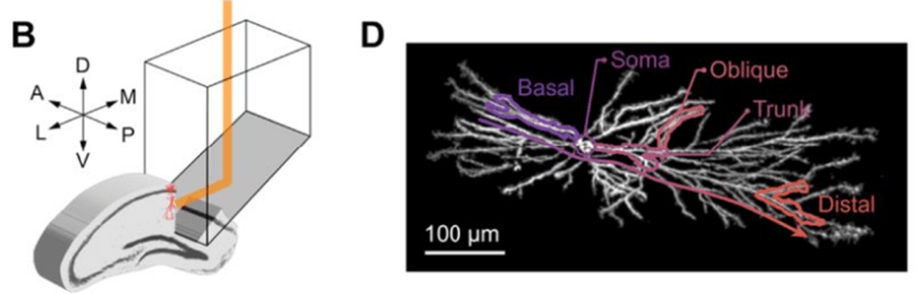
To achieve subcellular resolution for a single neuron in a living animal, that neuron must first be fluorescently labeled. Ideally, only that neuron would be targeted to avoid background fluorescence. This may be achieved using specialized viral strategies for sparse labeling (Jefferis and Livet, 2012), or by targeted single-cell electroporation (Gonzalez et al., 2025b). The next challenge is to simultaneously observe all of the neuron’s dendrites and spines and their activity. A typical layer 5 cortical neuron spans almost the entire cortical depth; in mice, its dendrites extend over more than 600 micrometers.

The only method that allows imaging at such depths in vivo with acceptable speed is two-photon microscopy (Helmchen and Denk, 2005). However, even two-photon microscopy is relatively slow, making it impossible to scan an entire dendritic tree at sufficient speed. Scanning speed is fundamentally limited by fluorescence lifetime (approx. 3 ns), preventing us from reaching the speeds required to sample a complete dendritic arbor (dendritic length of a single pyramidal cell: approx. 10’000 µm). Dedicated microscopes based on AOD scanners have been built for this purpose (Akemann et al., 2022; Grewe et al., 2010; Katona et al., 2012; Nadella et al., 2016), but none of them can scan 10 mm of dendritic length distributed across >600 micrometers at high speed. But not only the scan speed is limiting, but also the fluorescence yield: even if we managed to quickly scan across the entire dendrite and excite each point of the dendrite, we may not get a lot of fluorescence from it due to the low number of fluorophors. But, even though I play the devil’s advocate here, I have to admit that we’re not completely out of sight of the goal. And there are new scanning technologies (Demas et al., 2021; Zhong et al., 2025) that are not fully applicable for this purpose but make us aware that for neuroscience and microscopy the impossible might actually be possible in the future. And even now, we may be able to scan a substantial portion of a neuron’s dendritic tree (maybe 10% of it) at a reasonable speed.

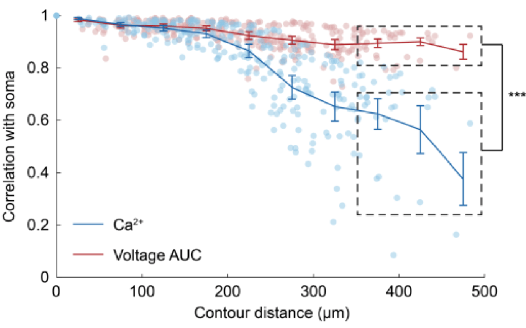
But let’s talk about the fluorophores and what they measure. The most commonly used fluorophores for this task are calcium indicators. They are relatively bright and slow, which makes them ideal to record across an entire neuron, where it takes some time to scan the entire dendritic tree. However, they primarily reflect the neuronal output (the action potential in the soma and axon, and the backpropagating action potential in the dendrites). Inputs in dendrites are often not seen at all, or overshadowed by the backpropagating action potential (Francioni et al., 2019). In spines, there are studies which show that inputs can be recorded without contamination by backpropagating action potentials (Iacaruso et al., 2017; Wilson et al., 2016), but these analyses still come with a lot of uncertainty and have been questioned by future experiments and analyses (Kerlin et al., 2019). Also, inhibitory synapses don’t come with spines and would therefore be missed entirely. New classes of sensors could fix this problem, detecting either glutamate (or GABA for inhibitory synapses) (Aggarwal et al., 2025; Kolb et al., 2025) or the membrane potential (voltage indicators) (Hao et al., 2024; Liu et al., 2022). These sensors are, however, faster, making it necessary to record at a repetition rate of almost 1000 Hz (or a bit lower for subthreshold events). With current sensors and two-photon recording modalities, it seems difficult to imagine performing such recordings for a entire dendritic tree, at high speed, high signal-to-noise, and at high spatial resolution. (Gonzalez et al., 2025a) published a study which comes closest to this ideal experiment and is definitely worth a read.

What we would learn:
The primary result would be a complete description of how a neuron processes synaptic information. How do synapses on the apical dendrite, hundreds of micrometers from the soma, influence the decision to fire an action potential? How linear or nonlinear is signal integration, really? These are straightforward, and maybe somewhat academic, questions that have remained unresolved for a long time (Stuart et al., 2016). But the implications of such an experimental dataset would go much further. By observing synaptic inputs over long periods, we could precisely determine how similar neighboring inputs are. In addition, and more importantly, we would see how activity patterns that do or do not coincide with somatic action potentials are strengthened or weakened over time. For example, if a synapse is repeatedly active but never supported by neighboring or spatially distant synapses, it should eventually weaken and be eliminated morphologically. But according to which exact rules does this remodeling occur? How many futile activations are required before weakening begins? Does weakening affect only that synapse, or neighboring ones as well? Such questions about coordinated plasticity of clustered synapses are already addressed at a smaller scale (Kastellakis and Poirazi, 2019; Larkum and Nevian, 2008; Ujfalussy and Makara, 2020), but they are hampered by incomplete pictures and contaminated readouts of inputs vs. outputs.

Overall, these research topics may sound like small details for scientists not working in this field, but it is precisely such details that define the generative rules governing neuronal function. Therefore, the major advance of this experiment would be the systematic exploration of many such rules – details that are currently known only sparsely or from isolated slice experiments. The result of this experiment would be a lexicon of rules describing how current neuronal activity shapes future input strength. In essence, these are the rules for the plasticity and learning of individual neurons. With these plasticity rules, we could understand the principles individual neurons follow as actors within a collective that performs intelligent information processing and storage.

Going conceptually slightly beyond that, the dataset would allow us to address questions that are currently out of reach. One such idea, which I have discussed previously on this blog, is that neuronal action potentials should be interpreted as actions of cells (with cells considered as agents); in this scheme, subsequent synaptic inputs would represent the feedback/reaction received, as described also elsewhere in more detail with the concept of individual neurons as control units(Moore et al., 2024). This perspective places the single neuron back at the center, framing the closed loop of action and reaction from the neuron’s point of view. An experiment that simultaneously records inputs and output of a single cell would make such ideas, which are currently untestable, empirically accessible.

References

Aggarwal, A., Negrean, A., Chen, Y., Iyer, R., Reep, D., Liu, A., Palutla, A., Xie, M.E., MacLennan, B.J., Hagihara, K.M., Kinsey, L.W., Sun, J.L., Yao, P., Zheng, J., Tsang, A., Tsegaye, G., Zhang, Y., Patel, R.H., Arthur, B.J., Hiblot, J., Leippe, P., Tarnawski, M., Marvin, J.S., Vevea, J.D., Turaga, S.C., Tebo, A.G., Carandini, M., Rossi, L.F., Kleinfeld, D., Konnerth, A., Svoboda, K., Turner, G.C., Hasseman, J.P., Podgorski, K., 2025. Glutamate indicators with increased sensitivity and tailored deactivation rates. Nat Methods. https://doi.org/10.1038/s41592-025-02965-z

Akemann, W., Wolf, S., Villette, V., Mathieu, B., Tangara, A., Fodor, J., Ventalon, C., Léger, J.-F., Dieudonné, S., Bourdieu, L., 2022. Fast optical recording of neuronal activity by three-dimensional custom-access serial holography. Nat Methods 19, 100–110. https://doi.org/10.1038/s41592-021-01329-7

Gonzalez, K.C., Negrean, A., Liao, Z., Terada, S., Zhang, G., Lee, S., Ócsai, K., Rózsa, B.J., Lin, M.Z., Polleux, F., Losonczy, A., 2025a. Synaptic basis of feature selectivity in hippocampal neurons. Nature 637, 1152–1160. https://doi.org/10.1038/s41586-024-08325-9

Gonzalez, K.C., Noguchi, A., Zakka, G., Yong, H.C., Terada, S., Szoboszlay, M., O’Hare, J., Negrean, A., Geiller, T., Polleux, F., Losonczy, A., 2025b. Visually guided in vivo single-cell electroporation for monitoring and manipulating mammalian hippocampal neurons. Nat Protoc 20, 1468–1484. https://doi.org/10.1038/s41596-024-01099-4

Grewe, B.F., Langer, D., Kasper, H., Kampa, B.M., Helmchen, F., 2010. High-speed in vivo calcium imaging reveals neuronal network activity with near-millisecond precision. Nat Methods 7, 399–405. https://doi.org/10.1038/nmeth.1453

Hao, Y.A., Lee, S., Roth, R.H., Natale, S., Gomez, L., Taxidis, J., O’Neill, P.S., Villette, V., Bradley, J., Wang, Z., Jiang, D., Zhang, G., Sheng, M., Lu, D., Boyden, E., Delvendahl, I., Golshani, P., Wernig, M., Feldman, D.E., Ji, N., Ding, J., Südhof, T.C., Clandinin, T.R., Lin, M.Z., 2024. A fast and responsive voltage indicator with enhanced sensitivity for unitary synaptic events. Neuron 112, 3680-3696.e8. https://doi.org/10.1016/j.neuron.2024.08.019

Helmchen, F., Denk, W., 2005. Deep tissue two-photon microscopy. Nat Methods 2, 932–940. https://doi.org/10.1038/nmeth818

Iacaruso, M.F., Gasler, I.T., Hofer, S.B., 2017. Synaptic organization of visual space in primary visual cortex. Nature 547, 449–452. https://doi.org/10.1038/nature23019

Jefferis, G.S., Livet, J., 2012. Sparse and combinatorial neuron labelling. Current Opinion in Neurobiology 22, 101–110. https://doi.org/10.1016/j.conb.2011.09.010

Kastellakis, G., Poirazi, P., 2019. Synaptic Clustering and Memory Formation. Front. Mol. Neurosci. 12, 300. https://doi.org/10.3389/fnmol.2019.00300

Katona, G., Szalay, G., Maák, P., Kaszás, A., Veress, M., Hillier, D., Chiovini, B., Vizi, E.S., Roska, B., Rózsa, B., 2012. Fast two-photon in vivo imaging with three-dimensional random-access scanning in large tissue volumes. Nat Methods 9, 201–208. https://doi.org/10.1038/nmeth.1851

Kerlin, A., Mohar, B., Flickinger, D., MacLennan, B.J., Dean, M.B., Davis, C., Spruston, N., Svoboda, K., 2019. Functional clustering of dendritic activity during decision-making. eLife 8, e46966. https://doi.org/10.7554/eLife.46966

Kolb, I., Hasseman, J.P., Matsumoto, A., Jensen, T.P., Kopach, O., Arthur, B.J., Zhang, Y., Tsang, A., Reep, D., Tsegaye, G., Zheng, J., Patel, R.H., Looger, L.L., Marvin, J.S., Korff, W.L., Rusakov, D.A., Yonehara, K., GENIE Project Team, Turner, G.C., 2025. iGABASnFR2: Improved genetically encoded protein sensors of GABA. https://doi.org/10.7554/eLife.108319.1

Larkum, M.E., Nevian, T., 2008. Synaptic clustering by dendritic signalling mechanisms. Current Opinion in Neurobiology 18, 321–331. https://doi.org/10.1016/j.conb.2008.08.013

Liu, Z., Lu, X., Villette, V., Gou, Y., Colbert, K.L., Lai, S., Guan, S., Land, M.A., Lee, J., Assefa, T., Zollinger, D.R., Korympidou, M.M., Vlasits, A.L., Pang, M.M., Su, S., Cai, C., Froudarakis, E., Zhou, N., Patel, S.S., Smith, C.L., Ayon, A., Bizouard, P., Bradley, J., Franke, K., Clandinin, T.R., Giovannucci, A., Tolias, A.S., Reimer, J., Dieudonné, S., St-Pierre, F., 2022. Sustained deep-tissue voltage recording using a fast indicator evolved for two-photon microscopy. Cell 185, 3408-3425.e29. https://doi.org/10.1016/j.cell.2022.07.013

Moore, J.J., Genkin, A., Tournoy, M., Pughe-Sanford, J.L., De Ruyter Van Steveninck, R.R., Chklovskii, D.B., 2024. The neuron as a direct data-driven controller. Proc. Natl. Acad. Sci. U.S.A. 121, e2311893121. https://doi.org/10.1073/pnas.2311893121

Nadella, K.M.N.S., Roš, H., Baragli, C., Griffiths, V.A., Konstantinou, G., Koimtzis, T., Evans, G.J., Kirkby, P.A., Silver, R.A., 2016. Random-access scanning microscopy for 3D imaging in awake behaving animals. Nat Methods 13, 1001–1004. https://doi.org/10.1038/nmeth.4033

Stuart, G., Spruston, N., Häusser, M. (Eds.), 2016. Dendrites. Oxford University Press. https://doi.org/10.1093/acprof:oso/9780198745273.001.0001

Ujfalussy, B.B., Makara, J.K., 2020. Impact of functional synapse clusters on neuronal response selectivity. Nat Commun 11, 1413. https://doi.org/10.1038/s41467-020-15147-6

Wilson, D.E., Whitney, D.E., Scholl, B., Fitzpatrick, D., 2016. Orientation selectivity and the functional clustering of synaptic inputs in primary visual cortex. Nat Neurosci 19, 1003–1009. https://doi.org/10.1038/nn.4323

Zhong, J., Natan, R.G., Zhang, Q., Wong, J.S.J., Miehl, C., Bose, K., Lu, X., St-Pierre, F., Guo, S., Doiron, B., Tsia, K.K., Ji, N., 2025. FACED 2.0 enables large-scale voltage and calcium imaging in vivo. Nat Methods. https://doi.org/10.1038/s41592-025-02925-7

Posted in Calcium Imaging, closed-loop, Imaging, neuroscience, Reviews | Tagged brain, Calcium Imaging, electrophysiology, Microscopy, neuroscience | 4 Comments

Annual report of my intuition about the brain (2025, part I)

Posted on December 27, 2025 by P.T.R. Rupprecht

During a talk in Basel in 1980, Sydney Brenner stated that “so much progress depends on the interplay of techniques, discoveries and new ideas, probably in that order of decreasing importance” (Brenner, 2002). This statement got converted into the famous quote: “Progress in science depends on new techniques, new discoveries, and new ideas, probably in that order”. What is missing from the famous quote is the word interplay. This omission highlights what scientific research truly needs, and something that proponents of technology development often forget to mention: technology needs to interact with scientific ideas and discoveries in order to become powerful.

Sometimes I get the impression that neurotechnology takes on a life of its own and is developed for its own sake. The fact that the ultimate goal of a specific technology is unattainable seem to discourage interaction with ideas, because those ideas are not within reach, and investments into technology alone seems therefore more reasonable. That is why I want to try today to think through what it would actually mean if we could indeed achieve three different seemingly unachievable experimental goals.

Here comes part I, with parts II and III following in a couple of days.

I. Reconstructing memories and mind from the connectome of a human brain

The idea:
Synaptic connections between neurons can be observed anatomically as long as the spatial precision is high enough, which can be achieved with electron microscopy that can achieve a resolution of a few nanometers. Other methods, such as expansion microscopy (Tavakoli et al., 2025) or X-ray tomography (Bosch et al., 2025), may provide similar resolution in the future, but the basic assumption does not change: the brain must already be dead (preferably not for too long). If it were possible to image an entire human brain with electron microscopy and detect all synapses and their strengths, we would obtain the (synaptic) connectome: all connections between all neurons, including their weights. Like an artificial neural network, this biology-derived network could then be run in a simulation, reconstructing the knowledge and experiential world of the dead brain. There is even a not-so-small community that hopes that such a method could grant them some form of life after death and, therefore, immortality.

Why it won’t work:
In principle, the method itself works very well. In 2025, connectomics was even named “Method of the Year” by Nature Methods (Marx, 2025). Over the past years, connectomics has provided fascinating insights into brain organization, particularly in simpler animals, most notably the fruit fly Drosophila. For the fruit fly, the connectome was approached five years ago (the “hemibrain” dataset) (Scheffer et al., 2020) and nearly completely reconstructed more recently (Dorkenwald et al., 2024; Lin et al., 2024; Matsliah et al., 2024; Schlegel et al., 2024). Since individual neurons are arranged almost identically from fly to fly, this catalog has become extremely useful for the entire fruit fly community.

So why shouldn’t this also work for a mammalian or human brain? For several reasons. First, the human brain is simply too large. Even imaging small brains or brain fragments is currently an enormous challenge. Producing a single high-quality, high-resolution 2D image of brain tissue is not particularly difficult. Maintaining that same quality across thousands, millions, or billions of images is. If we say that one image is 4096×4096 pixels, and we wanted to image at 10 nm resolution in x and y (the fruit fly connectomes use even higher resolutions) and in 20 nm slices in z, we would need to record roughly 10²⁰ imaging voxels for a 1-2 liter volume of human brain tissue, or 6 10¹² (or 6 trillion) images. Which is a lot of images that need to be acquired without mistakes! If even one small brain region hidden in a corner is not well captured, the entire idea of a complete connectome is called into question. Microscopes can fail due to power outages; cutting blades may drag a dust particle across the sample and scratch entire image series; heavy metals used for contrast may not penetrate certain brain regions well enough to reveal synapses. Any such high-precision methods are inherently fragile and error-prone, making them less scalable. When imaging a fruit fly brain, this is manageable – you can simply try again with another brain of another fly until the sample quality is sufficient and your software does not produce a critical crash. But if you want to reconstruct the connectome of a specific human, you get only one attempt.

Second, there is the issue of data analysis. Manually reconstructing a single human neuron takes several days, or, according to more optimistic views (which I do not share), a few hours. The human brain contains roughly 100 billion neurons. Who is supposed to do this work? AI, of course. There are already impressive methods for automated segmentation of neurons and detection of synapses. However, in all cases, manual validation is still required to correct false mergers and reassemble neurons that have been split during segmentation. Researchers have tried to automate this process (Celii et al., 2025; Schmidt et al., 2024), but in practice these steps are still mostly performed by humans. Could AI fully automate this time-critical step? Probably yes. Will it happen in the near future? At present, I see little concrete evidence, only preliminary prototypes and promises.

Third, an open question is how much we would actually learn from the connectome. How much information can be inferred from the anatomical appearance of a synapse? Can we tell which neurotransmitter it uses, or whether the synapse adapts or facilitates to incoming input? How can we reconstruct dynamic activity patterns from static synapses? Can we understand how a synapse on a spine interacts in terms of electrophysiologcally with the dendrite and soma based solely on an electron micrograph? How can we take into account molecular details such as voltage-gated ion channels and their distribution? All of these aspects are under active investigation, but they are far from being resolved. And it remains unclear (with unclear, I mean as unclear as in the halting problem) when they will be understood well enough so we can judge whether a purely anatomical connectome is sufficient to reconstruct memories and the inner life of a brain, be it human or not.

Based on these considerations, I still believe that connectomics is one of several essential methods in basic neuroscience, and certainly one of the most promising. But even if a connectomic anatomical reconstruction worked perfectly, it would not suddenly mean that we can wake up the mind from a dead brain with its dynamics.

What we would learn:
Suppose we could reconstruct all neurons in a human brain and detect all synapses, assigning each a weight that reflects its true functional strength (even though it is still unclear whether this is fully possible). We could systematically revisit and test many existing findings in neuroscience. For example, global connectivity in the human brain is often measured using diffusion tensor imaging (DTI), which relies on anisotropic diffusion of water molecules along fiber bundles. It would be both exciting and important to validate and refine this method using a connectome, improving accuracy by several orders of magnitude.

Even more importantly, a connectome would revolutionize research fields that focus on specific brain regions. For example, there are relatively large research communities for each of the major cortical and non-cortical brain areas such as the basolateral amygdala (processing of emotion and fear), the locus coeruleus (stress and arousal), or the hypothalamus (homeostasis and endocrine control). A recurring question is: where does this region actually receive its inputs from? For that, current neuroscience heavily relies on retrograde (virus) tracing, which labels neurons projecting to a given region. These methods are powerful but not fully reliable, as injections are difficult to restrict spatially, and viruses often have unexplained biases for or against certain neurons’ axons. A connectome would replace all such experiments in one stroke.

But it would go much further. We could examine not only the inputs to a region, but the inputs to those inputs – mapping the full receptive field of a region or even specific cell types. Conversely, we could finally understand the impact of a region or neuron: where do its axons project, and where do the axons of its downstream targets project? Analogous to a receptive area, we could map an impact field in a clear and systematic way.

With a connectome, many theories about the organization of brain regions could be decisively confirmed or discarded. With today’s relatively small datasets from animal experiments, this is already partially possible, though with major limitations, as shown, for example, in work from Moritz Helmstaedter’s lab, testing ideas such as predictive processing or the standard model of the cortical column (Sievers et al., 2024). For open questions like the importance of recurrent connectivity in the hippocampus or olfactory cortex, functional characterization of recurrence currently requires enormous effort with weak statistical power (Guzman et al., 2016; Layous et al., 2025). Right now, we have no good intuition about the prevalance of recurrent connections throughout brain areas and what kind of anatomical recurrences (single-synaptic loops, loops between thalamus and cortex, loops between specific cortical layers). Even a single connectome could clarify these issues immediately.

As with the fruit fly brain, such a dataset would be publicly accessible and would therefore constitute a reference for everyone, enabling any researcher or even interested laypeople to contribute not only ideas but also corrections, and thus making a big contribution to open science.

Overall, it is difficult to overstate the potential impact of a complete connectome. Yet, some scientists manage to do exactly that by claiming it would allow reconstruction of a person’s full memories. That remains far away and just as unrealistic as the promises made by the Blue Brain Project in the early 2000s. It is harder – but necessary – to explain to non-experts why the connectome would not deliver this result, and still be an absolute game changer.

References

Bosch, C., Aidukas, T., Holler, M., Pacureanu, A., Müller, E., Peddie, C.J., Zhang, Y., Cook, P., Collinson, L., Bunk, O., Menzel, A., Guizar-Sicairos, M., Aeppli, G., Diaz, A., Wanner, A.A., Schaefer, A.T., 2025. Nondestructive X-ray tomography of brain tissue ultrastructure. Nat Methods 22, 2631–2638. https://doi.org/10.1038/s41592-025-02891-0

Brenner, S., 2002. Life sentences: Detective Rummage investigates. Genome Biology 3.

Celii, B., et al., 2025. NEURD offers automated proofreading and feature extraction for connectomics. Nature 640, 487–496. https://doi.org/10.1038/s41586-025-08660-5

Dorkenwald, S., et al., 2024. Neuronal wiring diagram of an adult brain. Nature 634, 124–138. https://doi.org/10.1038/s41586-024-07558-y

Guzman, S.J., Schlögl, A., Frotscher, M., Jonas, P., 2016. Synaptic mechanisms of pattern completion in the hippocampal CA3 network. Science 353, 1117–1123. https://doi.org/10.1126/science.aaf1836

Layous, R., Tamás, B., Mike, A., Sipos, E., Arszovszki, A., Brunner, J., Szatai, Á., Yaseen, F., Andrási, T., Szabadics, J., 2025. Optical Recordings of Unitary Synaptic Connections Reveal High and Random Local Connectivity between CA3 Pyramidal Cells. J. Neurosci. 45, e0102252025. https://doi.org/10.1523/JNEUROSCI.0102-25.2025

Lin, A., Yang, R., Dorkenwald, S., Matsliah, A., Sterling, A.R., Schlegel, P., Yu, S., McKellar, C.E., Costa, M., Eichler, K., Bates, A.S., Eckstein, N., Funke, J., Jefferis, G.S.X.E., Murthy, M., 2024. Network statistics of the whole-brain connectome of Drosophila. Nature 634, 153–165. https://doi.org/10.1038/s41586-024-07968-y

Marx, V., 2025. Method of the Year: EM connectomics. Nat Methods 22, 2470–2475. https://doi.org/10.1038/s41592-025-02906-w

Matsliah, A., et al., 2024. Neuronal parts list and wiring diagram for a visual system. Nature 634, 166–180. https://doi.org/10.1038/s41586-024-07981-1

Scheffer, L.K., et al., 2020. A connectome and analysis of the adult Drosophila central brain. eLife 9, e57443. https://doi.org/10.7554/eLife.57443

Schlegel, P., et al., 2024. Whole-brain annotation and multi-connectome cell typing of Drosophila. Nature 634, 139–152. https://doi.org/10.1038/s41586-024-07686-5

Schmidt, M., Motta, A., Sievers, M., Helmstaedter, M., 2024. RoboEM: automated 3D flight tracing for synaptic-resolution connectomics. Nat Methods 21, 908–913. https://doi.org/10.1038/s41592-024-02226-5

Sievers, M., Motta, A., Schmidt, M., Yener, Y., Loomba, S., Song, K., Bruett, J., Helmstaedter, M., 2024. Connectomic reconstruction of a cortical column. https://doi.org/10.1101/2024.03.22.586254

Tavakoli, M.R., Lyudchik, J., Januszewski, M., Vistunou, V., Agudelo Dueñas, N., Vorlaufer, J., Sommer, C., Kreuzinger, C., Oliveira, B., Cenameri, A., Novarino, G., Jain, V., Danzl, J.G., 2025. Light-microscopy-based connectomic reconstruction of mammalian brain tissue. Nature 642, 398–410. https://doi.org/10.1038/s41586-025-08985-1

Posted in Data analysis, fMRI, Imaging, machine learning, Microscopy, Network analysis, Neuronal activity, neuroscience, Reviews | Tagged Data analysis, deep learning, machine learning, Microscopy, theoretical neuroscience | 4 Comments

Dirigo: a future Python alternative to Scanimage?

Posted on November 14, 2025 by P.T.R. Rupprecht

Over the last 20 years, many microscopes that are capable of resonant scanning two-photon microscopy have converged on using ScanImage, a powerful software package with many strengths but also two downsides: First, it is no longer open-source, and second, it is written in Matlab, a framework that many scientists and developers now find less attractive compared with more flexible languages such as Python. But how exactly would we replace ScanImage if we could design a microscope control software from scratch?

Screenshot from the Dirigo Demo (https://forum.image.sc/t/introducing-dirigo-post-2-demo-pipeline/115836).

Tim Weber has been working on these ideas. He has developed a framework called Dirigo that may serve as a modular, extensible backend for scientific image acquisition. One aspect of the design I particularly appreciate is its clean separation of responsibilities. Dirigo organizes its functionality into four independent “workers” – self-contained threads with a stop event and an inbox queue – which handle the core tasks of acquisition, processing, display, and logging. Based on my own experience building and rebuilding resonant-scanning microscope software (see my earlier blog post), this separation makes a great deal of sense. It not only creates components that can be flexibly combined, but also naturally distributes acquisition, computation, and visualization across threads. For anyone interested in online processing or closed-loop experiments, Dirigo’s structure looks like a very promising foundation.

If you’re curious and have a bit of time, take a look at the project on GitHub. Tim has also written a series of short posts on the Image.sc forum that go into the design in more detail:

I especially recommend posts #2 and #3. Post #2 includes a demo video and gives a clear explanation of how the worker model functions in practice. Post #3 digs into the digitizer interfaces, covering systems from National Instruments and Alazar to several boards I hadn’t encountered before but that look quite promising (and are also described in the GitHub README).

These and other hardware interfaces are a crucial part of any microscope control system, since they define how the software communicates with the acquisition hardware itself. If you’re interested in contributing – whether by adding wrappers for specific devices or by expressing interest in particular hardware interfaces – I am pretty sure that Tim would be very happy to hear from you!

Posted in Calcium Imaging, Imaging, Microscopy, neuroscience | Tagged Calcium Imaging, Microscopy, photons, Scanning, technology | Leave a comment

Interesting papers on astrocyte ultrastructure and function

Posted on November 14, 2025 by P.T.R. Rupprecht

Astrocytes are brain cells that are often completely overlooked and dismissed or, in the opposite extreme, presented as mysterious devices that somehow solve all problems of computational neuroscience. The truth is somewhere in the middle, but it is not clear yet where exactly. First of all, we still do not understand even the basic mechanistic rules by which individual astrocytes operate. For neurons, we have precise, often even mathematical ideas how they receive input via synapses, how they depolarize, and how depolarizations propagate to the soma and elicit action potentials. For astrocytes, this mechanistic book of rules is still missing – and this gap limits our ability to interpret experiments or build coherent theories.

As part of the effort to close this gap, some of my own research focuses on how astrocytes respond to neuromodulatory input and how they process these responses through subcellular calcium signals (Rupprecht et al., 2024). These signals depend not only on passive propagation – somewhat analogous to passive dendritic spread in neurons – but also on the fine astrocytic morphology (branches, branchlets, leaflets/perisynaptic astrocytic processes, and endfeet) and on the subcellular organelles (endoplasmic reticulum and mitochondria) that shape calcium dynamics.

Below, I highlight a few recent studies that may advance our understanding of astrocytic structure and function, and illustrate both how far we have come and how far we still need to go.

Synapses are partially wrapped by astrocytic processes

A central concept in astrocyte biology is the “tripartite synapse”. This describes the idea that a neuronal synapse, consisting of a presynapse and a postsynapse, is wrapped by a third component (hence the “tri”), an astrocytic process, creating a microenvironment where the astrocytic process interacts with the synaptic partner for neuronal plasticity, neurotransmitter clearance and maybe other purposes. However, it was not clear how much of the synaptic landscape is actually “covered” by astrocytic processes.

A recent study by Nam et al. (2025) reported that over 85% of synapses in the dentate gyrus of hippocampus have an astrocytic process within 120 nm of some part of the synaptic perimeter. This study comes from the Harris lab, which is worth mentioning since Kristen Harris was one of the key researchers to establish the concept of the tripartite synapse (Ventura and Harris, 1999). Another recent study by Yener et al. (2025) from the Helmstaedter lab examined synaptic coverage in mouse somatosensory cortex. This is how the 3D reconstruction of a tripartite synapse looks like (taken from Figure 1 of Yener et al. (2025), under CC BY-NC-ND 4.0 license):

Using a stringent criterion (“≥50% of synaptic perimeter covered by astrocytic membrane within 40 nm”), they found that only ~23% of synapses were wrapped by PAPs. At first glance, this seems surprisingly low, first compared to the concept of tripartite synapses, and second compared to the study by Nam et al. (2025), who reported much higher coverages.

But when we look more closely, we can see that this number heavily depends on the definition of “wrapping.” When the authors relaxed the distance and coverage criteria (e.g., 20% coverage within 100 nm), the proportion increased dramatically – up to ~78%, which would be again more consistent with the study by Nam et al. (2025). Yener et al. (2025) also provide this nice plot below to make these relationships transparent (taken from Figure 1 of Yener et al. (2025), under CC BY-NC-ND 4.0 license):

Therefore, the datasets are relatively consistent; what differs is how authors interpret which distances and coverage percentages are biologically meaningful – and this is an important point. Structural metrics are only interpretable in the context of hypotheses about how astrocytes interact with synapses and what temporal precision is required for that interaction.

On that note, it is interesting to see that both Yener et al. (2025) and Nam et al. (2025) relate their structural findings to synaptic plasticity. However, they use very different methods to infer or generate synaptic plasticity – using LTP and LTD protocols in slices by Nam et al. (2025), and co-variances of spine sizes by Yener et al. (2025), a method that was – interesting coincidence – partially established by Bartol et al. (2015), which was a collaboration where Kristen Harris’ lab contributed the experimental part. Back to Yener et al. (2025) and Nam et al. (2025): The results from the two approaches about synaptic coverage as a function of LTD vs. LTP are, unfortunately, not really consistent, and there are too many possible reasons for the differences to be worth discussing. It will in any case require additional future work to get a clear picture.

Multiple astrocytic processes combine to wrap multiple synapses

A study that challenges our textbook view of astrocyte-synapse interactions is by Benoit et al. (2025) from the labs of Karin Pernet-Gallay and Andrea Volterra. This study directly questions the concept of the “tripartite synapse” – where the idea is that a functional unit is formed by one presynaptic terminal, one postsynaptic terminal, and one astrocytic process wrapping around.

Astrocytes form small processes (10-20 nm) that are called “leaflets” or, when wrapping around neuronal synapses, “perisynaptic astrocytic processes (PAPs)”. These astrocytic processes are too small to be resolved by light microscopy but can be identified by electron microscopy. Benoit et al. use large-volume electron microscopy to demonstrate that the smallest astrocytic processes (leaflets/PAPs) do not primarily wrap individual synapses but instead form multi-leaflet networks that, connected via gap junctions, ensheath groups of 1–20 synapses. This is a very interesting finding that might change how we think about ensembles of synapses and how they may be controlled as a group of synapses by mediation of this shared ensheathing by a common leaflet, forming – as the authors put it – a “tripartite synaptic network”. Here is an example from their paper which nicely illustrates the idea – even though the choice of colors is one of the worst I have ever seen for color-blind people like me, with leaflets in green, axonal boutons in yellow, spine in orange and synaptic cleft in red (from Figure 2 of Benoit et al., 2025, under the CC BY 4.0 license):

With their analysis, they also add a data point to the question of “astrocytic coverage” discussed above. Consistent with the interpretation of Yener et al. (2025), they find low coverage of synapses by individual leaflets – however, they find that the majority of synapses receives a larger “astrocytic coverage” by a larger ensheathing by multiple leaflets.

Benoit et al. (2025) go one step further, attempting to image functional signals in leaflets vs. calcium signals in other processes of astrocytes. Because leaflets are too small to resolve with standard in vivo imaging, the authors used a creative indirect approach. Since mitochondria are absent from leaflets but present in larger astrocytic processes, they image mitochondrial markers in a secondary channel and can thus infer which calcium signals originated from leaflet vs. non-leaflet regions. This approach, of course, cannot deliver the same precision as electron microscopy, but is a very interesting tool to functionally dissect subcellular structures in astrocytes. For more details, check out the paper – it is worth it.

Astrocytes as mediators of neuromodulatory feedback

A final recent study I would like to mention is by Xin et al. (2025) from the lab of Hailan Hu. It is not about ultrastructural properties but about the function of astrocytes in brain-wide circuits. Hailan Hu’s lab is well-known for their expertise on the lateral habenula and its role in depression. Here, they pull off an impressive array of experiments (fiber photometry, pharmacological and genetic perturbations of cell types or signaling pathways, behavior, etc.) that could have easily been several distinct and interesting papers.

Their main observation is that the lateral habenula (LHb) is activated (based on fiber photometry) before many other brain regions during stress. This activity in turn switches on the locus coeruleus (LC), which is known to project to a large part of the brain including cortex and hippocampus – where I have studied its long-range effects on astrocytes (Rupprecht et al., 2024), and where slice work indicates that these activated astrocytes release ATP/adenosine and thereby inhibit neurons in CA1 (Lefton et al., 2025). But LC also projects back to LHb, where it also activates astrocytes. Interestingly, Xin et al. (2025) observe that these astrocytes not only release adenosine but also glutamate, which results in a net activation of LHb neurons in a second wave. This claim is, however, not as solidly supported by the data as it appears at first glance: In Figure 4k (which I cannot show here due to copyright restrictions), Xin et al. (2025) test multiple antagonists against glutamate receptors, adenosine receptors, GABA receptors, etc. They see a small reduction after superfusing the antagonist, which is, however, only significant for glutamate, ATP-R and A2AR antagonists. Each of those experiments is done with 2-3 slices, but they perform statistics based on single cells. Of course, one would expect batch effects between slices, and the actual power of the experiment is much lower than reported. This is a common fallacy that can be seen in most papers. The proper way to deal with this statistical problem would be to use hierarchical statistics, for example based on linear mixed-effect models.

Despite these minor concers, I still find it a very interesting study, full of many advanced technical approaches. Personally, I would have preferred to go in much more depth for individual experiments with more detailed analyses. As they are, many results are only minimally discussed (due to space constraints). They nicely act as puzzle pieces within the bigger story. But they are not dicussed – and with “discussed”, I mean “analyzed” – beyond this limited horizon of interest. To give an example, Xin et al. (2025) use complex behaviors such as foot shocks to elicit stress responses; but it would have been interesting to simultaneously monitor motor and other behavior to better relate the temporal components of the neuronal responses to what is going on with the animal. But I can understand why it also makes sense to condense this massive amount of diverse experiments into a single paper in order to highlight the story and the main finding. In any case, if you work on astrocytes or locus coeruleus, this is a must-read.

References

Bartol, T.M., Bromer, C., Kinney, J., Chirillo, M.A., Bourne, J.N., Harris, K.M., Sejnowski, T.J., 2015. Nanoconnectomic upper bound on the variability of synaptic plasticity. eLife 4, e10778. https://doi.org/10.7554/eLife.10778

Benoit, L., Hristovska, I., Liaudet, N., Jouneau, P.-H., Fertin, A., De Ceglia, R., Litvin, D.G., Di Castro, M.A., Jevtic, M., Zalachoras, I., Kikuchi, T., Telley, L., Bergami, M., Usson, Y., Hisatsune, C., Mikoshiba, K., Pernet-Gallay, K., Volterra, A., 2025. Astrocytes functionally integrate multiple synapses via specialized leaflet domains. Cell 188, 6453-6472.e16. https://doi.org/10.1016/j.cell.2025.08.036

Lefton, K.B., Wu, Y., Dai, Y., Okuda, T., Zhang, Y., Yen, A., Rurak, G.M., Walsh, S., Manno, R., Myagmar, B.-E., Dougherty, J.D., Samineni, V.K., Simpson, P.C., Papouin, T., 2025. Norepinephrine signals through astrocytes to modulate synapses. Science 388, 776–783. https://doi.org/10.1126/science.adq5480

Nam, A.J., Kuwajima, M., Parker, P.H., Bowden, J.B., Abraham, W.C., Harris, K.M., 2025. Perisynaptic Astroglial Response to In Vivo Long-Term Potentiation and Concurrent Long-Term Depression in the Hippocampal Dentate Gyrus. J. Neurosci. 45, e0943252025. https://doi.org/10.1523/JNEUROSCI.0943-25.2025

Rupprecht, P., Duss, S.N., Becker, D., Lewis, C.M., Bohacek, J., Helmchen, F., 2024. Centripetal integration of past events in hippocampal astrocytes regulated by locus coeruleus. Nat Neurosci 27, 927–939. https://doi.org/10.1038/s41593-024-01612-8

Ventura, R., Harris, K.M., 1999. Three-Dimensional Relationships between Hippocampal Synapses and Astrocytes. J. Neurosci. 19, 6897–6906. https://doi.org/10.1523/JNEUROSCI.19-16-06897.1999

Xin, Q., Wang, J., Zheng, J., Tan, Y., Jia, X., Ni, Z., Xu, Z., Feng, J., Wu, Z., Li, Y., Li, X.-M., Ma, H., Hu, H., 2025. Neuron-astrocyte coupling in lateral habenula mediates depressive-like behaviors. Cell 188, 3291-3309.e24. https://doi.org/10.1016/j.cell.2025.04.010

Yener, Y., Motta, A., Helmstaedter, M., 2025. Connectomic analysis of astrocyte-synapse interactions in the cerebral cortex. https://doi.org/10.1101/2025.02.20.639274

Posted in Astrocytes, Calcium Imaging, Data analysis, Microscopy, neuroscience, Reviews | Tagged Calcium Imaging, Microscopy, neuroscience, science | Leave a comment

I never meant to study the brainstem

Posted on September 25, 2025 by P.T.R. Rupprecht

I was recently invited to contribute a guest post on Substack by Vijay Iyer – some years ago one of the main developers of ScanImage in the lab of Karel Svoboda, and more recently a strong advocate for ME/CFS awareness and for communication pathways between brain and body. Earlier this year, we had a series of conversations about circuit neuroscience and the potential of dissecting brainstem circuits. Here’s my write-up on substack, where I describe why I believe that brainstem nuclei may be ideal targets for brain-interfaces, in particular when interfacing (indirectly) with astrocytes: I never meant to study the brainstem.

Posted in Astrocytes, Brain machine interface, Calcium Imaging, hippocampus, Locus coeruleus, Microscopy, writing | Tagged arousal, brain, Calcium Imaging, Microscopy, neuroscience, photons, science, stress | Leave a comment

	P.T.R. Rupprecht on Hippocampal neuron and astrocy…
	Anonymous on Hippocampal neuron and astrocy…
	P.T.R. Rupprecht on Annual report of my intuition…
	Anonymous on Annual report of my intuition…
	P.T.R. Rupprecht on Annual report of my intuition…
	Anonymous on Annual report of my intuition…
	Annual report of my… on Annual report of my intuition…
	Annual report of my… on Annual report of my intuition…
	Annual report of my… on Annual report of my intuition…

	P.T.R. Rupprecht on Hippocampal neuron and astrocy…
	Anonymous on Hippocampal neuron and astrocy…
	P.T.R. Rupprecht on Annual report of my intuition…
	Anonymous on Annual report of my intuition…
	P.T.R. Rupprecht on Annual report of my intuition…
	Anonymous on Annual report of my intuition…
	Annual report of my… on Annual report of my intuition…
	Annual report of my… on Annual report of my intuition…
	Annual report of my… on Annual report of my intuition…

A blog about neurophysiology

Subcellular calcium and voltage imaging of pyramidal neurons in mouse hippocampus

Paper 1: Two-photon random-access voltage and calcium imaging of CA1 dendrites

Online motion correction for fast dendritic two-photon imaging

Decoupling of calcium vs. voltage with higher dendritic branch order

Local dendritic voltage signals

Paper 2: Prism-based one-photon voltage imaging of CA1 dendrites

One-photon voltage imaging of individual CA1 neurons

A note on data analysis

Anti-correlation of apical vs. basal dendrite activity

Evidence against prominent local voltage events in dendrites

Backpropagation enhanced by local depolarization

Paper 3: Simultaneous calcium and voltage imaging across the dendritic tree

One-photon imaging of voltage and calcium in individual neurons

A biophysical rule to convert voltage to calcium

Further evidence against prominent local events in dendrites

Conclusion

References

CascadeTorch: a PyTorch version of Cascade for spike inference

What is Cascade?

Why switch to PyTorch?

What is CascadeTorch?

Compatibility and support

A clearing method for large human FFPE tissue blocks

Hippocampal neuron and astrocyte responses to noradrenaline and natural arousal

Annual report of my intuition about the brain (2025, part III)

Annual report of my intuition about the brain (2025, part II)

Annual report of my intuition about the brain (2025, part I)

Dirigo: a future Python alternative to Scanimage?

Interesting papers on astrocyte ultrastructure and function

I never meant to study the brainstem

Recent Comments

Recent Posts

Archives

Categories

Recent Comments