One of the most amazing methods in modern neuroscience is dense volumetric electron microscopy of the brain. I have mentioned some openly accessible datasets before (see my previous blog post), but many additional datasets have been released since then – most prominently from drosophila, but also from zebra finch, zebrafish, mouse, and even the human brain.
My own research in the lab is primarily focused on the hippocampus, so I am always specifically curious about hippocampal datasets. There’s a relatively old one by Bloss et al. (2018) obtained from mouse hippocampus. However, when I saw a new hippocampal dataset published earlier this year, I was quite intrigued. This new dataset, described by Corteze et al. (2025) in a preprint from Helene Schmidt‘s lab in Frankfurt, was acquired in “coronal” slices, resembling how the rodent hippocampus (or at least dorsal CA1) is often visualized in standard histology. This acquisition modality clearly reveals the hippocampal layers, making it easy to navigate, even for non-experts not familiar with electron microscopy data. You can browse the dataset just by clicking for example on this link: https://wklink.org/7023
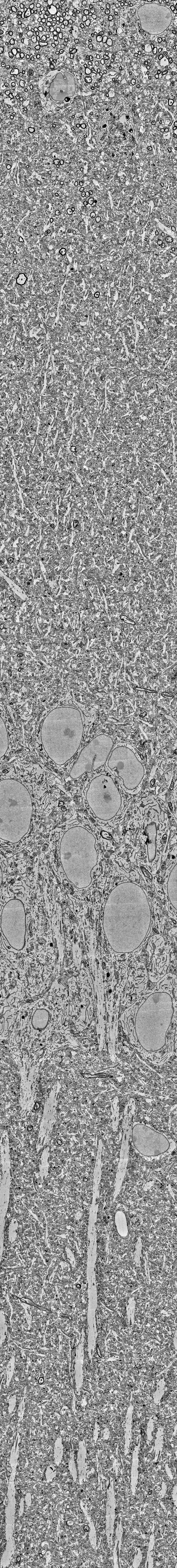
The layering of the hippocampus that can be seen in these images is really beautiful (see picture below). At the top, you see the myelinated axons of the corpus callosum, then the small dendrites of the stratum oriens, then the dense layer of pyramidal neurons’ cell bodies. Going further, you can clearly trace the huge apical dendrites of pyramidal cells – if you ever wondered why apical dendrites are visible even under regular light microscopy while smaller dendrites are not, here is your answer. What a beautiful layering; and how difficult to visualize without extensive scrolling!
Derived from the dataset published by Corteze et al. (2025), downloaded from the server using a custom-written script which you can find on GitHub.
Unfortunately, all the fine details like small dendrites, axon myelin sheaths or mitochondria are barely visible when you zoom out on a normal screen; and the overall architecture of the hippocampus, in return, becomes hard to see when you zoom in. To visualize both scales, I decided to print out the hippocampal “column” and use it to decorate a small section of my office wall.
Downloading the data takes a bit of coding. A screen capture doesn’t work because the data browser adapts the resolution of the currently rendered view (using a multi-resolution pyramid data format). So, I wrote a small script (on GitHub) which downloads one single coronal imaging plane from the server to my own hard disk. (Downloading the whole dataset would be prohibitive due to its size.) Then I selected the hippocampal “column” that I wanted to have on my walls.
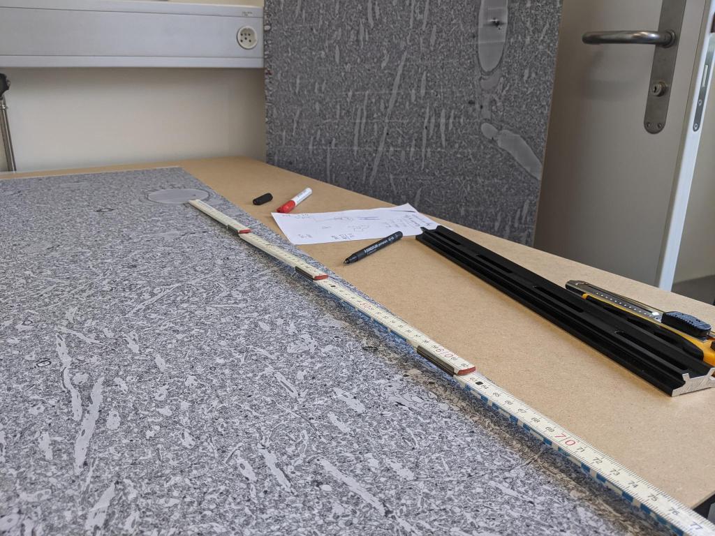
Next, I printed the hippocampal EM image as a poster – actually, it was three A0 posters to span the full height of my office, which is over 3 meters. To stabilize the posters, I glued them onto thin wooden panels bought from a local hardware store.
Next, I measured the boundaries of the surrounding walls and doors to make the panels fit into the shapes of walls, door, and ceiling. Stefan Giger and Martin Wieckhorst, who have access to a bench saw at the institute, kindly cut the panels to make them fit into the space. I covered the connecting edges where two panels met with black insulation tape, and used short nails to attach the panels to the walls.
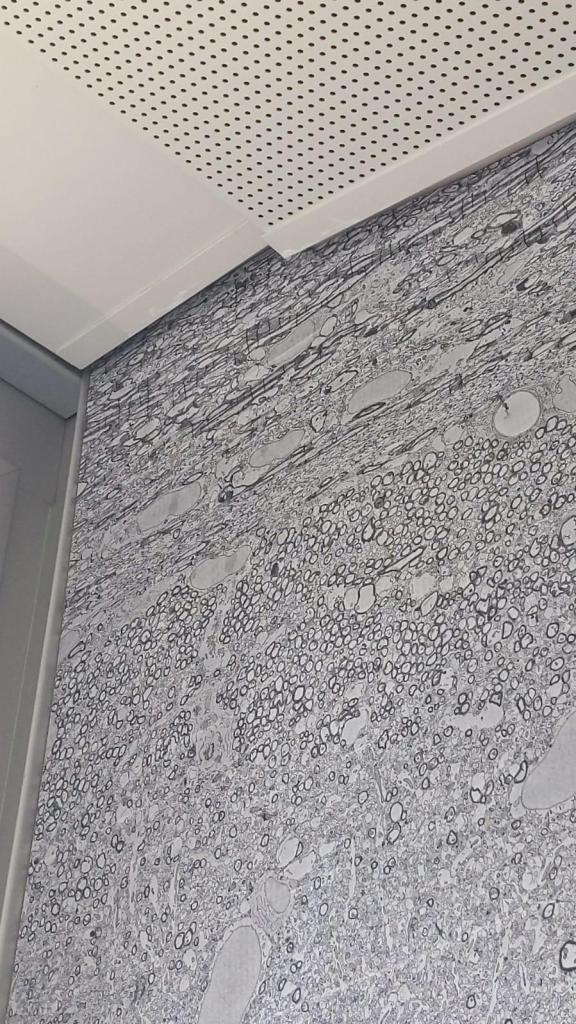
For the next iteration, I would probably use a more expensive glossy print. However, overall I’m quite happy with the result. Here’s a glimpse of how the corpus callosum with its myelinated axons nicely fits the ceiling:
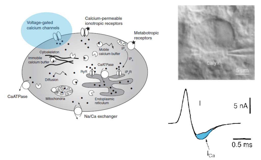
Many researchers, including myself, use calcium imaging to read out the activity of neurons in the living brain. This method relies on the fact an action potential – the “spike” of neuronal activity – opens voltage-gated calcium channels, transiently increasing the calcium concentration in the cell.
Calcium influx during action potentials, mediated by voltage-gated calcium channels. Left: Scheme of calcium-related processes in neurons. Right: Electrophysiological measurement of calcium current influx upon an action potential in the Calyx of Held. Figure with excerpts from Gerard et al. (1998) and Helmchen (2012).
However, calcium isn’t just an indicator of action potentials; it’s a seemingly universal signaling molecule used in most if not all living cells on Earth. In neurons, calcium concentration is also influenced by influx from cell organelles, in particular the endoplasmatic reticulum (ER, a loose web that is weaved through the cytoplasm) and the mitochondria (the “powerhouse” of the cell). These organelles are present not only in the cell body but also in its dendrites and axons. As an expert for calcium imaging (check out my latest work on calcium sensors) with a long-standing interest in dendrites, I thought it would make sense to have a glimpse into the current literature on calcium signals coming from neuronal cell organelles. Here are three papers from the last years that I selected to read more carefully – but I’m happy to receive pointers to additional ones that might be equally relevant!
Calcium signaling at junctions between plasma membrane and endoplasmic reticulum
This paper might be especially interesting for you if you are curious about the role of dendritic spines. In this impressive study, Benedetti et al. (2025) investigate the structural basis of a key player for calcium signaling in neuronal dendrites, the endoplasmic reticulum (ER). They use an amazing array of techniques, from super-resolution lattice light sheet microscopy, volumetric electron microscopy, dual-color calcium imaging in cytosol and ER, extensive pharmacology, to two-photon glutamate uncaging – there is something for almost everybody.
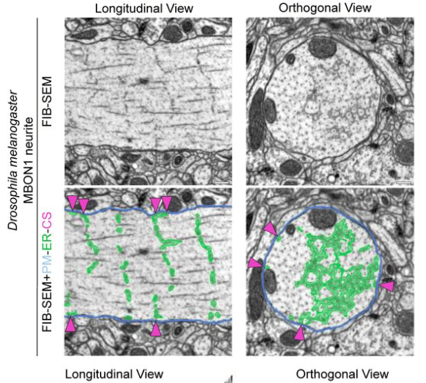
Their main finding is that the ER forms regular junctions with the plasma membrane, spaced by 1 μm, while the rest of the ER is floating in the cytosol like a weave (see figure excerpt below).
The ladder-like structure of the endoplasmic reticulum (ER, green) in cross-sections of dendrites, imaged with high-resolution volumetric electron microscopy (FIB-SEM). Excerpt of Figure 2 from the preprinted paper, under CC BY-NC-ND 4.0 license.
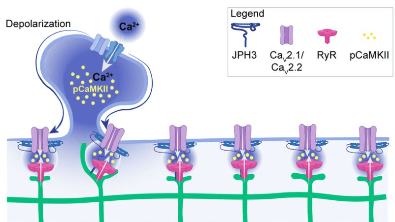
Benedetti et al. show that these junctions are also functionally relevant because they concentrate specific calcium channels and result in local activation of CaMKII. Maybe the most important aspect: The ER can reach into spine heads, and activation of single spines can propagate as calcium signal within the ER up to 20 μm along the dendrite. This observation is important since dendritic spines have often been speculated to be distinct compartments that are, by virtue of the high spine neck resistance, insulated from the neighboring dendritic compartment (that’s still a matter of debate). Here, Benedetti et al. show that the ER can bypass this insulation, not by electrotonic propagation but by calcium signaling.
In summary, a very beautiful paper – where spatially resolved cell biology meets neuroscience.
Suggested scheme of calcium signaling from a spine that propagates along the dendrite through the endoplasmic reticulum (ER) and activates calcium channels (Cav2.1, Cav2.2) locally at junctions of the ER with the plasma membrane. Excerpt of Figure 7 from the preprinted paper, under CC BY-NC-ND 4.0 license.
Cytosolic calcium signals couple only loosely to mitochondrial calcium in vivo
In this interesting work, Lin et al. (2019) study the relationship between cytosolic and mitochondrial calcium signals in the intact mouse brain. To this end, they use dual color-imaging with the green calcium indicator GCaMP expressed in mitochondria and the red-shifted indicator RCaMP in the cytosol.
Previous work from cultured neurons or slices had suggested that there is tight coupling between mitochondrial and cytosolic calcium transients, but these findings were based on artificial stimulation. Here, Lin et al. find a less reliable coupling, with only 3-10% of cytosolic transients being reflected in mitochondrial calcium signaling, with the fraction depending on the processing load of the respective cortical areas (visual or motor cortex). This loose coupling during natural conditions is interesting and also raises the question to which extent artificial stimulation – e.g., the glutamate uncaging experiments performed by Benedetti et al. – relates to physiological stimulation levels.
Lin et al. find a couple of variables to explain which events are coupled and which ones are not. Yet, they conclude that the coupling seems still quite random (“probabilistic”). However, they find that CamKII, a self-phosphorylating kinase also involved in neuronal plasticity, is necessary to enable such coupling.
Another interesting point: Lin et al. find that mitochondrial calcium signals are not limited to small compartments but are synchronized across separate mitochondrial compartments across >15 μm. Since these compartments are only connected by small “nano-tunnels” of the ER, it is likely that calcium signals do not propagate across mitochondrial compartments but are orchestrated by a hidden global factor that could not be clearly observed during this study.
Intracellular calcium release shapes plasticity and place cells in hippocampus
O’Hare et al. (2022) investigate how intracellular calcium release from organelles affects dendritic and calcium signals and plasticity in hippocampal neurons of awake mice.
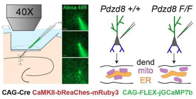
The key method of this study is single-cell in vivo electroporation, which enables the targeted insertion of plasmids for 1) expression of a calcium indicator, 2) expression of an optogenetic actuator, and 3) activation of a conditional knockout in a single visually targeted pyramidal cell. This method is described in more detail in this recent paper by Gonzalez et al., 2025 from the same lab.
Single-cell, two-photon targeted in vivo electroporation to express the optogenetic activator bReaChes, the calcium indicator jGCaMP7b, and to induce the cell-specific deletion of a protein related to mitochondria-ER coupling. Excerpt of Figure 1 from the preprinted paper, under CC BY-NC-ND 4.0 license.
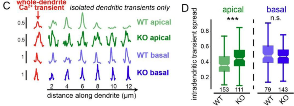
By genetically knocking out a gene responsible for ER-mitochondria coupling (Pdzd8), O’Hare et al. showed that the spatial extent of calcium signaling across the apical dendrites became more widespread (see figure excerpt below). This is a significant finding because extent of calcium signaling coupling between dendritic segments has been a long-standing question that is still not well-understood. This study shows that the functional coupling of intracellular organelles directly influences how calcium signals are compartmentalized within dendrites. In addition, the study demonstrates that this change of intradendritic spread of calcium signals is accompanied by functional plasticity (place cell properties; see the paper for details).
Knockout of the gene of interest increases the coupling length of calcium signals along the apical but not basal dendrite of hippocampal pyramidal neurons. Excerpt of Figure 4 from the preprinted paper, under CC BY-NC-ND 4.0 license.
Conclusion
In summary, these papers show an important part of neurons that is often completely forgotten by systems neuroscientists – the cellular biology. A reason why such results are ignored is that they are often obtained in cell cultures or similar artificial systems where the cell organelles and stimulation patterns can be quite different. Lin et al., for example, demonstrate that the tight coupling of mitochondrial to cytosolic calcium is not observed in vivo, underlining the importance of research done in vivo.
A second aspect why there are few such studies is their technical difficulty. Obtaining clean and interpretable signals from two different calcium indicators as done by Lin et al. is very challenging (but see Moret et al., 2025 for the promising development of the chemigenetic sensor HaloCaMP specifically for mitochondria and ER). Similarly, the in vivo electroporation technique by O’Hare et al. is definitely a highly challenging method that I haven’t seen used widely.
Another method where I see a lot of potential for future analyses of cell organelle function in neuronal dendrites is volumetric high-resolution electron microscopy. Existing datasets that are publicly available might contain important information about the interplay of endoplasmic reticulum, mitochondria, the plasma membrane, and the cytosol. Maybe we only need to ask the right question.
.
References
Benedetti, L., Fan, R., Weigel, A.V., Moore, A.S., Houlihan, P.R., Kittisopikul, M., Park, G., Petruncio, A., Hubbard, P.M., Pang, S., Xu, C.S., Hess, H.F., Saalfeld, S., Rangaraju, V., Clapham, D.E., De Camilli, P., Ryan, T.A., Lippincott-Schwartz, J., 2025. Periodic ER-plasma membrane junctions support long-range Ca2+ signal integration in dendrites. Cell 188, 484-500.e22. https://doi.org/10.1016/j.cell.2024.11.029
Gerard, J., Borst, G., Helmchen, F., 1998. Calcium influx during an action potential, in: Methods in Enzymology. Elsevier, pp. 352–371. https://doi.org/10.1016/S0076-6879(98)93023-3
Gonzalez, K.C., Noguchi, A., Zakka, G., Yong, H.C., Terada, S., Szoboszlay, M., O’Hare, J., Negrean, A., Geiller, T., Polleux, F., Losonczy, A., 2025. Visually guided in vivo single-cell electroporation for monitoring and manipulating mammalian hippocampal neurons. Nat Protoc 20, 1468–1484. https://doi.org/10.1038/s41596-024-01099-4
Helmchen, F., 2012. Calcium imaging, in: Brette, R., Destexhe, A. (Eds.), Handbook of Neural Activity Measurement. Cambridge University Press, pp. 362–409. https://doi.org/10.1017/CBO9780511979958.010
Lin, Y., Li, L.-L., Nie, W., Liu, X., Adler, A., Xiao, C., Lu, F., Wang, L., Han, H., Wang, X., Gan, W.-B., Cheng, H., 2019. Brain activity regulates loose coupling between mitochondrial and cytosolic Ca2+ transients. Nat Commun 10, 5277. https://doi.org/10.1038/s41467-019-13142-0
Moret, A., Farrants, H., Fan, R., Zingg, K., Gee, C.E., Oertner, T.G., Rangaraju, V., Schreiter, E.R., De Juan-Sanz, J., 2025. An expanded palette of bright and photostable organellar Ca2+ sensors. https://doi.org/10.1101/2025.01.10.632364
O’Hare, J.K., Gonzalez, K.C., Herrlinger, S.A., Hirabayashi, Y., Hewitt, V.L., Blockus, H., Szoboszlay, M., Rolotti, S.V., Geiller, T.C., Negrean, A., Chelur, V., Polleux, F., Losonczy, A., 2022. Compartment-specific tuning of dendritic feature selectivity by intracellular Ca2+ release. Science 375, eabm1670. https://doi.org/10.1126/science.abm1670
Interneurons are inhibitory neurons in the brain that are thought to shape the computations performed by principal cells. The effects of inhibition can be rather diverse, depending on which neurons – or which parts of a neuron (dendrites, soma, or the axon hillock) – are targeted. A particularly interesting inhibitory motif that is the disinhibitory motif, which depends on a specific interneuron type known as VIP neuron. VIP neurons primarily inhibit another interneuron type called SST neurons (also written as “‘SOM”), which in turn inhibits principal or pyramidal cells, often by targeting their dendrites. Therefore, activating VIP neurons releases pyramidal neurons from SST-mediated inhibition, possibly creating a window for plasticity and learning.
Unfortunately, both VIP and SST neurons are not homogeneous classes but consist of multiple subtypes which might also vary across cortical and neocortical areas. Below, I’ll highlight a few recent studies on VIP neurons that caught my attention. Let me know if you know others that are similarly interesting!
A role for hippocampal VIP neurons in place cell remapping
In this well-designed and easy-to-read paper, Neubrandt, Lenkey et al. (2025) from the Vervaeke lab investigate how VIP neurons in the hippocampus contribute to place cell remapping. Place cell remapping is a form of hippocampal plasticity where pyramidal cells change their spatial firing fields in response to environmental novelty.
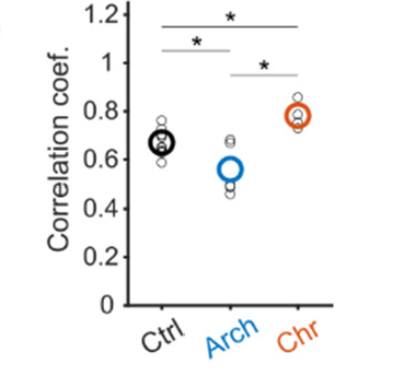
Neubrandt, Lenkey et al. use optogentic tools to activate (ChrimsonR) and inactivate (ArchT) VIP neurons while performing calcium imaging of pyramidal neurons. They find that inactivation decreases remapping and activation increases remapping of pyramidal neurons. The effects are relatively subtle but seem convincing, and align with the idea that VIP neurons facilitate plasticity by disinhibiting pyramidal neurons.
Effect of activating or inactivating VIP neurons on pyramidal neuron patterns. From Neubrandt, Lenkey et al. (2025), under CC BY 4.0 license (Figure 2L).
The authors additionally analyze their data with respect to a specific plasticity rule in pyramidal cells termed behavioral timescale synaptic plasticity (covered before on this blog), which results in a more complex picture that is less straightforward to interpret. The authors conclude that in addition to VIP activity other factors (e.g., neuromodulatory input) may be necessary to induce remapping.
Overall, this study nicely shows how novelty activates VIP interneurons to help control plasticity in pyramidal neurons, presumably via SST neurons. Their findings are consistent with and extend previous results from Turi et al. (2019) that demonstrated a necessary role of VIP neurons for reward location learning in hippocampal place cells.
The subtypes of VIP neurons in neocortex
Dellal, Zurita et al. (2025) from Bernardo Rudy’s lab investigate subtypes of VIP neurons in neocortex (somatosensory cortex). They do so in a very systematic study with transgenic animal crossing strategies that enable identification of various subtypes. I really do not want to know how much work it was to cross and validate all these mouse lines! As a result, Dellal, Zurita et al. find four subtypes of VIP neurons.
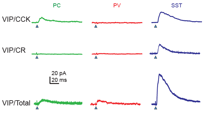
The most distinctive feature of these subtypes is whether the protein CCK is expressed or not. CCK-negative VIP neurons and in particular CCK-negative CR-positive VIP neurons target mostly SST neurons, while CCK-positive VIP neurons target also pyramidal cells directly and are there not only disinhibitory but also inhibitory for pyramidal cells. It is interesting that very similar findings have been made earlier for hippocampal circuits, where two such subtypes of VIP neurons were found in the 1990s (Acsády et al., 1996; Gulyás et al., 1996).
Effect for VIP subtypes on different hippocampal neuron types. From Dellal, Zurita et al. (2025), under CC BY 4.0 license (Figure 4B).
With the increasingly refined functional classification of interneuron subtypes, it becomes more and more difficult to not get confused by the different classification approaches. Other studies (e.g., in Figure 7 by Geiller et al., 2020) used slightly different markers to delineate VIP subclasses, making it quite a puzzle to connect the dots between publications!
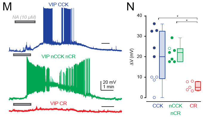
A detail that I found particularly interesting as somebody working on the noradrenergic system is the following finding: CR-positive VIP neurons, which target SST neurons but not pyramidal neurons, were not significantly activated by bath-applied noradrenaline (Fig. 6M,N); this is suprising because I would have expected noradrenalin to have a disinhibitory effect on the local circuit and therefore to act via VIP-CR interneurons – which does not seem to be the case. CCK-positive VIP cells as well as CCK-negative CR-negative VIP neurons (the fourth class found by the authors) were, however, activated by noradrenaline. So maybe all the disinibitory action through noradrenaline goes through CCK-negative CR-negative neurons? This definitely needs more follow-up experiments. I would be very curious to see these same experiments done in hippocampus …
Response of VIP subtypes towards bath-application of noradrenaline. From Dellal, Zurita et al. (2025), under CC BY 4.0 license (Figure 6M,N).
The main take-away from this paper is quite clear: perturbations of VIP neurons using transgenic VIP lines do affect multiple subtypes with partially opposing signature, with both disinhibitory effects (via CCK-negative interneurons) and inhibitory effects directly on pyramidal cells (via CCK-positive interneurons). This confound from using VIP transgenic lines is also discussed by the above study of Neubrandt, Lenkey et al., (2025). Targeting interneurons more specifically seems essential for future studies to manipulate or replicate the disinhibitory effect of (a subset of) VIP neurons, in neocortex as well as in hippocampus.
Hippocampal interneurons with all-optical methods
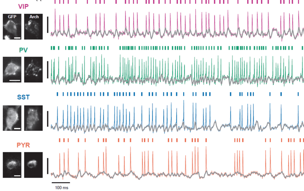
In an beautiful technical achievement, Yang et al. (2025) from Yoav Adam’s lab provide a systematic study of the functional characteristics of different neuron types in hippocampus (principal cells, VIP, SST, PV). They combine 1P voltage imaging (with the voltage sensors somArchon1 and QuasAr6b) and optogenetic activation of the same neurons (somCheRiff) to both record and manipulate specific neurons in vivo. Pretty cool! I liked how they focused on recording from and perturbing only very few neurons at a time, but at a apparently high quality.
Voltage imaging from various cell types in mouse hippocampus in vivo. From Yang et al. (2025), under CC BY 4.0 license (Figure 1C).
To describe these results, the authors analyze how optogenetic depolarization as well as state (walking vs. quiet) influences several cellular characteristics: the response to input, the amplitude of theta oscillations, and – for pyramidal neurons – the bursting propensity.
In a second step, Yang et al. use modeling to better interpret these descriptive findings. These single-cell conductance-based models are interesting to consider and consistent with the experimental results. However, I believe that the data itself and its pure description remain the strongest part of the paper. Such a dataset with voltage recordings and perturbations of several cell types in hippocampus would have been difficult to imagine just 10 or 15 years ago. I sincerely hope that the dataset will be curated and shared openly during the publication process!
.
References
Acsády, L., Görcs, T.J., Freund, T.F., 1996. Different populations of vasoactive intestinal polypeptide-immunoreactive interneurons are specialized to control pyramidal cells or interneurons in the hippocampus. Neuroscience 73, 317–334. https://doi.org/10.1016/0306-4522(95)00609-5
Dellal, S., Zurita, H., Kruglikov, I., Valero, M., Abad-Perez, P., Geron, E., Meng, J.H., Prönneke, A., Hanson, J.L., Mir, E., Ongaro, M., Wang, X.-J., Buzsáki, G., Machold, R., Rudy, B., 2025. Inhibitory and disinhibitory VIP IN-mediated circuits in neocortex. https://doi.org/10.1101/2025.02.26.640383
Geiller, T., Vancura, B., Terada, S., Troullinou, E., Chavlis, S., Tsagkatakis, G., Tsakalides, P., Ócsai, K., Poirazi, P., Rózsa, B.J., Losonczy, A., 2020. Large-Scale 3D Two-Photon Imaging of Molecularly Identified CA1 Interneuron Dynamics in Behaving Mice. Neuron 108, 968-983.e9. https://doi.org/10.1016/j.neuron.2020.09.013
Gulyás, A.I., Hájos, N., Freund, T.F., 1996. Interneurons Containing Calretinin Are Specialized to Control Other Interneurons in the Rat Hippocampus. J. Neurosci. 16, 3397–3411. https://doi.org/10.1523/JNEUROSCI.16-10-03397.1996
Neubrandt, M., Lenkey, N., Vervaeke, K., 2025. VIP interneurons control hippocampal place cell remapping through transient disinhibition in novel environments. https://doi.org/10.1101/2025.02.01.636072
Turi, G.F., Li, W.-K., Chavlis, S., Pandi, I., O’Hare, J., Priestley, J.B., Grosmark, A.D., Liao, Z., Ladow, M., Zhang, J.F., Zemelman, B.V., Poirazi, P., Losonczy, A., 2019. Vasoactive Intestinal Polypeptide-Expressing Interneurons in the Hippocampus Support Goal-Oriented Spatial Learning. Neuron 101, 1150-1165.e8. https://doi.org/10.1016/j.neuron.2019.01.009
Yang, Q., Baror-Sebban, S., Kipper, R., London, M., Adam, Y., 2025. All-optical electrophysiology reveals behavior-dependent dynamics of excitation and inhibition in the hippocampus. https://doi.org/10.1101/2025.03.20.644347
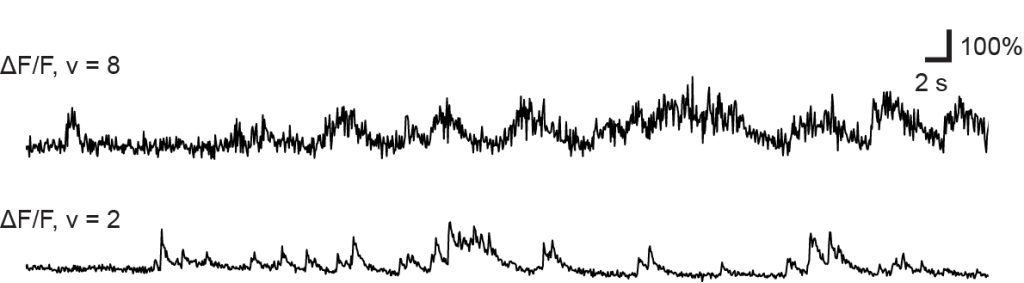
It is fascinating how much data quality can vary between different calcium imaging data sets. In this blog post, I will discuss a metric to quantify and compare data quality and in particular shot noise between calcium imaging datasets.
This variation of data quality depends on potential artifacts due to movement or instrument noise, the frame rate of the microscope, and the flux of fluorescence photons. The photon flux determines the shot noise level for each neuron and therefore whether calcium transients due to action potentials can be detected from the recording. Photon flux depends on factors such as neuron size (in pixels), indicator expression levels, and baseline brightness. As a result, it varies not only between recordings but also across neurons within the same session.
Two example ΔF/F traces from neurons of high (“8”) and low (“2”) standardized noise levels. Examples taken and modified from Rupprecht et al. (2025), under CC BY 4.0 license.
In our 2021 study on spike inference from calcium imaging data with CASCADE (Rupprecht et al., 2021), we took advantage of the fact that the slow calcium signal is typically very similar between adjacent frames. Therefore, the noise level can be approximated by
The median excludes outliers due to fast onset dynamics of calcium signals. Normalization by the square root of the frame rate makes the metric comparable across datasets with different frame rates. (I have discussed the application of this metric to various datasets in an earlier blog post.)
However, this metric is to some degree biased, as it assumes the ideal scenario of zero neuron activity. In the presence of neuronal activity, however, the ups and downs of calcium transients will increase the apparent noise level systematically. Recently, David Hildebrand brought up this issue, and I decided to look into it more carefully.
I used ground-truth spike patterns from electrophysiological recordings of cortical pyramidal neurons (mouse visual cortex, see Fig.2 Suppl.1), convolved them with a linear calcium kernel, and added Gaussian noise of known magnitude. Then, I quantified how precisely was able to recover the true noise value.
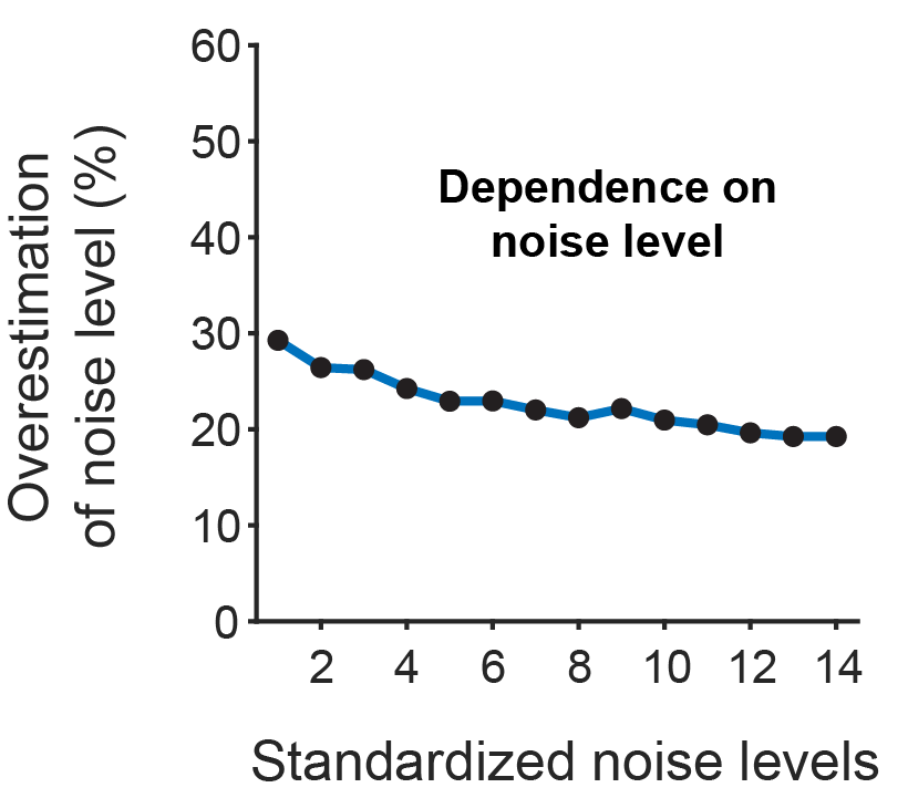
First, the metric generally overestimated the true noise level by about 20%. This overestimation was largely independent of the noise level but slightly increased for lower noise level. This makes sense: the relative effect of the same amount of a fixed level of neuronal activity is greater when the baseline noise is zero. However, the overall effect was relatively small – 20% is not dramatic for such a coarse metric:
Second, for low frame rates, the overestimation became more substantial, reaching up to 50% on average for a frame rate of 1-2 Hz. This is a significant bias that should be kept in mind. If you use the metric to quantitatively compare between recordings of different frame rates. it may be good to correct for this bias. In most other cases, this effect is likely negligible:
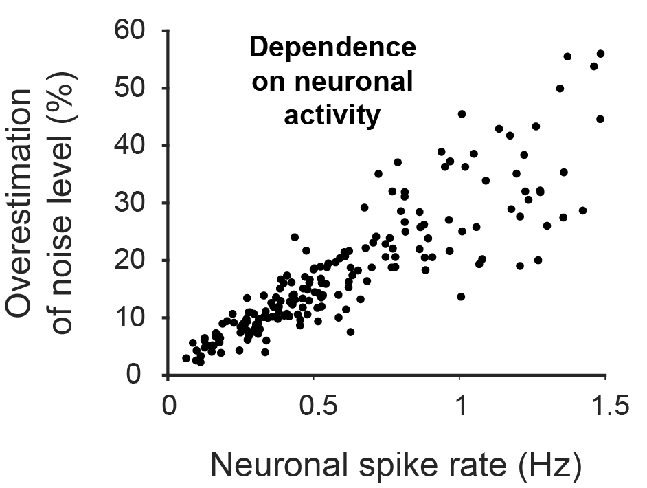
Finally, the overestimation also depended on the true spike rate of the respective recording. In the plot below, each point represents the quantification derived from the ground truth recording of an individual neuron with a its specific spike rate. As one would expect, the overestimation of noise levels is minimial for neurons that are almost silent, and grows almost linearly with the true spike rate:
Altogether, I still believe that the standardized noise level is a very useful (and probably under-used) metric to compare data quality across recordings. The above analyses provide context that should ideally be considered for quantitative comparisons – by quantifying how much the metric is affected by noise level, frame rate and individual spike rate.
Are you a finishing Master’s student with a quantitative background and are interested in neuroscience? This is your opportunity.
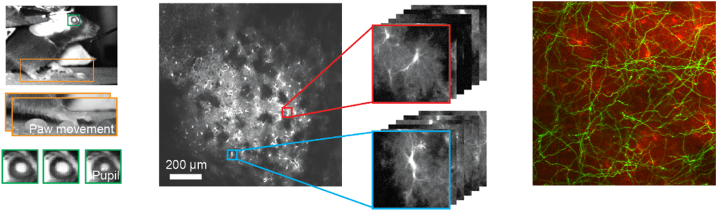
Project: You will be supervised by Dr. Peter Rupprecht and Prof. Fritjof Helmchen at the Brain Research Institute, University of Zurich. The project will be to study animal behavior in mice (left) together with the dynamics of subcellular calcium signals in neurons and astrocytes (middle), and how they are controlled by axonal projections from the brainstem (right). The activation of astrocytes is important for arousal and stress and therefore also for stress-related disorders. You will study the biological principles underlying subcellular activation of astrocytes, building upon previous work (Rupprecht et al., Nat Neuro, 2024). In a second branch of the project, you will study the role of astrocytes for memory consolidation and neuronal oscillations in a joint project with an optics engineer in the lab. Of course, there will always be possibilities to adapt projects to your specific skills.
Scope: You will learn how to use high-end two-photon microscopes to image the activity of neurons and astrocytes in the brain of a living animal. You will analyse large datasets in Python and/or Matlab. You will build models of subcellular signal integration to explain your experiments. You will have the opportunity to become creative and develop new methods for data analysis or microscopy. You will receive direct guidance from an expert on new methods for calcium imaging and data analysis (Peter Rupprecht) and from an experienced and world-reknown professor of neuroscience (Fritjof Helmchen).
Requirements: You have a background in physics, biophysics, neuronal engineering, or another quantitative discipline, and you are interested in performing neurophysiological experiments as well as extensive analyses and modeling.
Application: Please send your application including a CV and your transcript of records to Peter Rupprecht (rupprecht [snailsymbol] hifo.uzh.ch). Please include a letter of motivation that covers the following aspects: What talents or previous experience of yours are possibly relevant to this project? If you have coding or experimental experience, what was your most challenging previous program or project so far?
Many neuroscientists use calcium imaging to record the activity from neurons (or other cells in the brain). The video below was recorded by Sian Duss and me in hippocampal CA1 pyramidal cells in mice.
To make calcium imaging traces comparable across cells and recordings, most researchers use a method called ΔF/F (“delta F over F”) to normalize the fluorescence traces. However, there are different ways to compute ΔF/F, and it is not always obvious how to choose the best method and how to interpret the result.
Calcium imaging is used to record the activity of neurons in living animals. Often, these activity patterns are analyzed after the experiments to investigate how the brain works. Alternatively, it is also possible to extract the activity patterns in real time, decode them and control a device or computer with them. Such brain-computer-interface (BCI) or closed-loop paradigms have one important limiting factor: the delay between the neuronal activity and the control that this activity exerts over the device or computer.
For calcium imaging, this delay comprises the time to record the calcium images from the brain, but it is also limited by the slowness of calcium indicators. How are calcium indicators limiting such an online processing step in practice? And how is this limitation potentially mitigated by the family of GCaMP8 indicators, which have been shown to exhibit faster rise times than previous genetically indicators (<10 ms)?
We addressed this question using a supervised algorithm for spike inference (CASCADE), which extracts spiking information from calcium transients. We slightly redesigned the algorithm such that it only has access to a small fraction of the time after the time point of interest:
Spike inference using ony a few frames after the time point of interest (“Time after AP”). From Rupprecht et al, 2025, under CC BY 4.0 license (Figure 5c).
This modification of the algorithm was very simple since it is a simple 1D convolutional network, and we simply shifted the receptive field in time very slightly. The time defined in the scheme, which we call “integration time”, determines the delay for closed-loop application like BCI paradigms for calcium imaging. To achieve a very good performence in inferring the spiking activity from calcium signals, an integration time of 30-40 ms was required for GCaMP8 and 50-150 ms for GCaMP6.
Time after AP (see scheme above) to reach 90% of the maximal performance for spike inference. From Rupprecht et al, 2025, under CC BY 4.0 license (Figure 5d).
The CASCADE models trained for online spike inference are available online on our GitHub repository. The model names are starting with an “Online”, are listed as usual in this text file, and can be used as any other CASCADE models. For example, you can perform spike inference with your normal CASCADE model, and then perform the same spike inference with an “online” model, which will give you an impression how well the model performs. The only difference is that the “online” model takes only a few time points from the future, while the regular CASCADE model uses typically 32 time points from the future.
What does “a few time points” mean? Let’s look at a model’s name to break this down, for example the model Online_model_30Hz_integration_100ms_smoothing_25ms_GCaMP8. This model is trained for calcium imaging data acquired at 30 Hz with the calcium indicators GCaMP8 (the ground truth consisted of all GCaMP8 variants), with a smoothing of 25 ms. The crucial parameter is the integration time, here indicated as 100ms. This means that the model uses 100 ms from the future, which is 3 frames for the 30 Hz model.
If you are not sure which model to select for your application, or if you need another pretrained model for online spike inference, just drop me an email or open an issue for the GitHub repository.
For more details about the analysis and how the best choice of integration time for online spike inference depends on the noise levels of the calcium imaging recordings or potentially also other conditions such as calcium indicator induction methods or temperature, check out our recent preprint, where we also analyzed several other aspects of spike inference with a specific focus on GCaMP8: Spike inference from calcium imaging data acquired with GCaMP8 indicators.
There are two mutually exclusive holy grails of calcium imaging: First, recording from the highest number of neurons simultaneously. Second, detecting spike patterns with single-spike precision. This blog post focuses on the latter.
Many studies have claimed to demonstrate single-spike detection, but often only under specific conditions or for a subset of neurons. At the same time, nearly as many other studies have demonstrated that such single-spike detection is not possible under their respective conditions.
In our recent preprint, we’ve added systematic analyses based on ground truth recordings as our contributions to this debate. Specifically, we analyzed how single-spike detection depends on calcium indicators (GCaMP8s, GCaMP8m, GCaMP8f; GCaMP6f, GCaMP6m; XCaMP-Gf) and on the noise levels of the recordings.
What I particularly like about our approach is that it does not rely on arbitrary thresholds for false-positive vs. false-negative detections of action potentials. Instead, we trained a deep network (CASCADE) to predict spiking activity in general – optimizing for mean squared error loss when compared to ground truth spike rates.We then applied this network to individual single spike-related calcium transients, allowing us to quantify single-spike detection across calcium indicators and noise levels.
Fraction of correctly detected single, isolated action potentials. From Rupprecht et al, 2025, under CC BY 4.0 license (Figure 4e).
Calcium indicators are used to report the calcium concentration inside single cells. In neurons, calcium imaging can be used as a readout of neuronal activity (action potentials). However, some calcium indicators like GCaMP transform the calcium concentration of a cell into a fluorescence trace in a non-linear manner, following a sigmoidal curve:
Nonlinear relationship between the calcium concentration and the fluorescence of the calcium indicator. From Rupprecht et al, 2025, under CC BY 4.0 license (Figure 3a). Scheme loosely inspired by Rose et al. (2014).
This means that a small change in calcium concentration (ΔC1) may increase the fluorescence (ΔF1) only slightly, while the same change at a higher starting calcium concentration (ΔC2) leads to a much more prominent increase (ΔF2).
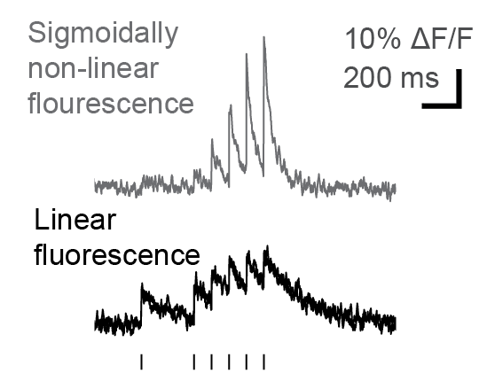
What many people do not consider is that this property has an effect on complex events with multiple bursts or action potentials in a sequence. The first spikes may only elicit small fluorescence changes, while the later spikes – with a large fraction of calcium ions still bound to the calcium indicators – result in much higher fluorescence changes. As a consequence, this results in a history-dependent bias that underestimates the early and overestimates the late phases of neuronal activity, as demonstrated with these simulated data:
Simulated fluorescence traces for non-linear sigmoidal (top, gray) and linear (bottom, black) transfer curves. From Rupprecht et al, 2025, under CC BY 4.0 license (Figure 3d).
It is striking to see that for the non-linear calcium indicator, the first spike is barely visible, while the later ones are disproportionally amplified compared to the linear fluorescence trace.
Such history-dependent effects are also important to keep in mind when comparing the neuronal activity dynamics across calcium indicators. GCaMP6f, for example, is highly non-linear, showing a strong history-dependent effect. GCaMP8m, on the other hand, seems to behave more linearly in cortical pyramidal neurons. Therefore, dynamics of complex events cannot be compared across these calcium indicators without taking these effects into account. And spike inference (e.g., using CASCADE) must also take these history-dependent effects into account!


 makes the metric comparable across datasets with different frame rates. (I have discussed the application of this metric to various datasets in an
  was able to recover the true noise value.