This is a blog post dedicated to those who start with calcium imaging and wonder why their live images seem to drown in shot noise. The short answer to this unspoken question: that’s normal.

Introduction

Two-photon calcium imaging is a cool method to record from neurons (or other cell types) while directly looking at the cells. However, almost everyone starting with their first recording is disappointed by the first light they see – because the images looked better, with more detail, crisper and brighter in Figure 1 of the lastest paper. What these papers typically show, is, however, not a snapshot of a single frame, but a carefully motion-corrected and, above all, averaged recording.

In reality, it is often not even necessary to see every structure in single frames. One can still make efficient use of such data that seemingly drown in noise, and you do not have to necessarily resort to deep learning-based denoising to make sense of the data. Moreover, if you can see your cells very clearly in a single frame, it is in many cases even likely that either the concentration of the calcium indicator or the applied laser power is too high (both extremes can induce damage and perturb the neurons).

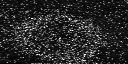
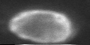
To demonstrate the contrast between typical single frames before and beautiful images after averaging for presentations, here’s a gallery of recordings I made. On the left, a single imaging frame (often seemingly devoid of any visible structure). On the right, an averaged movie. (And, yes, please read this on a proper computer screen for the details, not on your smartphone.)

Hippocampal astrocytes in mice with GCaMP6s

Here, I imaged hippocampal astrocytes close to the pyramidal layer of hippocampal CA1. Laser power: 40 mW, FOV size: 600 µm, volumetric imaging rate: 10 Hz (3 planes), 10x Olympus objective. From our recent study on hippocampal astrocytes, averaged across >4000 frames:

Pyramidal cells in hippocampal CA1 in mice with GCaMP8m

Here, together with Sian Duss, I imaged hippocampal pyramidal cells. Laser power: 35 mW, FOV size: 600 µm, frame rate: 30 Hz , 10x Olympus objective. Unpublished data, averaged across >4000 frames:

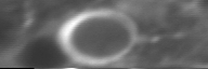
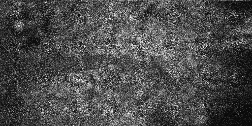
A single interneuron in zebrafish olfactory bulb with GCaMP6f

An interneuron recorded in the olfactory bulb of adult zebrafish with transgenically expressed GCaMP6f. Laser power <20 mW, 20x Zeiss objective, galvo-galvo-scanning. (Not shown: simultaneously performed cell-attached recording.) This is from the datasets that I recorded as ground truth for spike inference with deep learning (CASCADE). Zoomed in to a single isolated interneuron, averaged across 1000 frames:

A single neuron in zebrafish telencephalic region aDp with GCaMP6f

A neuron recorded in the telencephalic region “aDp” in adult zebrafish with transgenically expressed GCaMP6f. Laser power <20 mW, 20x Zeiss objective, galvo-galvo-scanning. (Not shown: simultaneously performed cell-attached recording.) This is from the datasets that I recorded as ground truth for spike inference with deep learning (CASCADE). Zoomed in to a single neuron, averaged across 1000 frames:

Population imaging in zebrafish telencephalic region aDp with GCaMP6f

Neurons recorded in the telencephalic region “aDp” in adult zebrafish with transgenically expressed GCaMP6f. Laser power <30 mW, 20x Zeiss objective, frame rate 30 Hz. Unpublished data, averaged across >1500 frames:

Sparsely labeled neurons in the zebrafish olfactory bulb with GCaMP5

Still in love with this brain region, the olfactory bulb. Here with sparse labeling of mostly mitral cells with GCaMP5 in adult zebrafish. This is one out of 8 simultaneously imaged planes, each imaged at 3.75 Hz, with this multi-plane scanning microscope. From our study where we showed stability of olfactory bulb representations of odorants (as opposed to drifting representations in the olfactory cortex homolog), averaged across 200 frames:

Population imaging in zebrafish telencephalic region pDp with OGB-1

Using an organic dye indicator (OGB-1), injected in and imaged from the olfactory cortex homolog in adult zebrafish. This is one out of 8 simultaneously imaged planes, imaged at 7.5 Hz each with this multi-plane scanning microscope. OGB-1, different from GECIs like GCaMP, comes with a relatively high baseline and a low ΔF/F response. The small neurons at the top not only look tiny, they are indeed very small (diameter typically 5-6 um). Unpublished data, averaged across 200 frames:

Pyramidal cells in hippocampal CA1 in mice with R-CaMP1.07

These calcium recordings from pyramidal neurons in hippocampal CA1 exhibited non-physiological activity. Laser power: 40 mW, FOV size: 300 µm, 16x Nikon objective, frame rate 30 Hz. From our recent study on pathological micro-waves in hippocampus upon virus injection, averaged across >1500 frames:

Conclusion

I hope you liked the example images! Also, I hope that this comparison across recordings and brain regions will help to normalize expectations about what to get from a single frame from functional calcium imaging. If you are into calcium imaging, you have to learn to love the shot noise!

And you have to learn to understand the power of averaging to be able to judge your image quality. Only averaging can truly reveal the quality of the recorded images. If the image remains blurry after averaging thousands of frames, then the microscope can indeed not resolve the structures. However, if the structures come out very clearly after averaging, the microscope’s resolution (and the optical access) are most likely good, and only the low amount of photons is stopping you from seeing signals clearly in single frames (which is often, as this gallery demonstrates, not even necessary).