‘Style transfer’ is a method based on deep networks which extracts the style of a painting or picture in order to transfer it to a second picture. For example, the style of a butterfly image (left) is transferred to the picture of a forest (middle; pictures by myself, style transfer with deepart.io):

Early on I was intrigued by these results: How is it possible to clearly separate ‘style’ and ‘content’ and mix them together as if they were independent channels? The seminal paper by Gatys et al., 2015 (link) referred to a mathematically defined optimization loss which was, however, not really self-explanatory. In this blog post, I will try to convey the intuitive step-by-step understanding that I was missing in the paper myself.

The resulting image (right) must satisfy two constraints: Content (forest) and style (butterfly). The ‘content’ is well represented by the location-specific activations of the different layers of the deep network. For the ‘style’, Gatys et al. suggest to calculate the joint activation patterns, i.e., correlations between activation patterns of different feature maps. These correlation matrices are mathematically speaking the Gram matrices of the network layers. This means that the Gram matrices of the butterfly image (left) and of the resulting style-transferred image (right) should be optimized to be as similar as possible. But what does this Gram matrix actually mean? Why does this method work?

A slightly better understanding comes with an earlier paper of Gatys et al. on texture synthesis (link). From there it becomes clear that the Gram matrix does not appear from nowhere but is inspired by comparably old-fashioned texture synthesis papers, especially by Portilla and Simoncelli, 2000 (link). This paper deals with the statistical properties that define what humans perceive consistently as the same texture, and the key word here is ‘joint statistics’. More precisely, they argue that it is not sufficient to look at the distributions of features (like edginess or other simple filters), but at the joint occurrence of features. This could be high spatial frequencies (feature 1) co-occurring with horizontal edges (feature 2). Or small spirals (feature 1) co-occurring with a blue color (feature 2). Co-occurences can be intuitively quantified by using the spatial correlation between each pair of feature maps correlations, since correlations are simply a measure of similarity between two (or more) things. As an important side-effect of the inner product associated with the correlation, the Gram matrix is invariant to the positions of features, which makes sense in the context of textures.

On a sidenote, Portilla and Simoncelli are not the first to have had a close look at joint statistics of textures. This is going back at least to Béla Julesz (1962), who conjectured that two images with the same second order statistics (= joint statistics) have textures that are indistinguishable for humans. (Later, he disproved his own conjecture based on counterexamples, but the idea of using joint statistics for texture synthesis remained useful.)

In old-school texture synthesis, features were handcrafted and carefully selected. When working with deep networks, features are much more numerous: they are simply the activation patterns of the layers. Each layer of a deep network consists not only of a single representation or feature map, but many of them (up to 100s or 1000s). Some are locally activated by edges, others by colors or parallel lines, etc. For the visualizations shown below, I’ve set up a Jupyter notebook to make it as transparent as possible. All of it is based on a GoogLeNet, pre-trained on the Imagenet dataset. Here are the feature maps (= activation patterns) of four input pictures (four columns). Green indicates high activation, blue low activation.

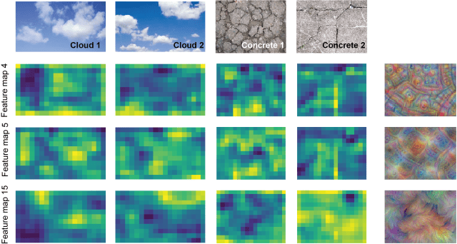
For the textures of cracked concrete, the feature maps 4 and 5 (second and third rows) are very similar to each other (correlated) and 15 is highly dissimilar (anti-correlated). Feature map 15 seems to have learned to detect large, bright and smooth surfaces like clouds. Therefore, the Gram matrix entry for the feature pair [4,5] will be consistently high for input images of cracked concrete, but low for cloud images. These are only few examples, but I think it makes pretty clear why correlations of feature maps are a better indicator of a texture than the simple mean activation of single feature maps.

To complement this analysis, I generated an input on the right-most column that optimizes the activation of the respective layers (see below for an explanation how I did this). Whereas feature maps 4 and 5 show edges and high-frequency structures, feature map 15 seems to prefer smooth textures.

Next, let’s have a look at how a full-blown Gram matrix looks like! But which layer would choose for this analysis?  I’m using a variant of the Inception network/GoogLeNet here, which seems to be a little bit less well-suited for style transfer than the VGG network typically used for style transfer. To find out a layer that is indicative of style, I applied 20 images of cloud textures and 20 images of cracked concrete. Then I measured both the confusion matrix of the Gram matrices for each layer, allowing to find the layer that optimally distinguishes these two textures (it is layer ‘mixed4c_3x3_pre_relu/conv’, more details are in the Jupyter notebook). As inputs, I have used greyscale images to prevent the color channels from dominating similarity measurements.

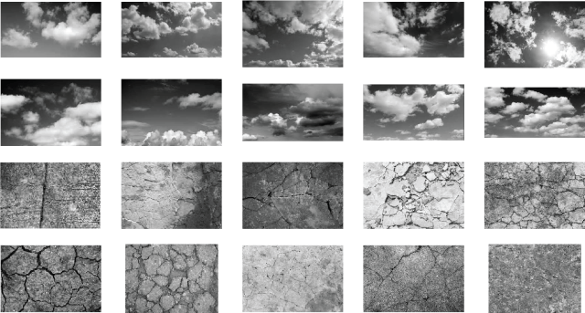
For the 16 inputs above, here come the 16 corresponding 256×256 Gram matrices of the chosen layer, arising from 256 feature maps. To clarify the presentation, I have rearranged the features in the matrices to highlight the clustering. The x- and y-axes of each matrix can be interpreted as the features of this layer, and the clustering highlights some of the feature similarities.

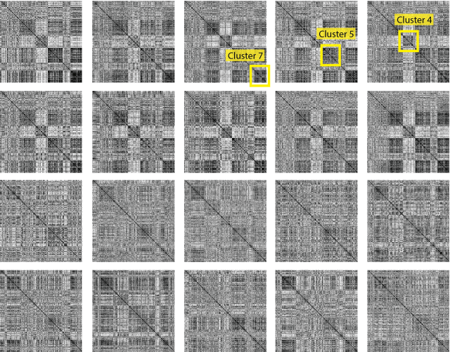
From that, it is quite clear that all cloud pictures display similar Gram matrices. The lower two rows with pictures of cracked concrete exhibit a more or less common pattern as well, which in turn is distinct from the cloudy Gram matrices.

As is clearly visible, the feature space is rather large. Therefore, since the contribution of single features is small, it does not make sense to look e.g. at a single feature pair that is highly correlated for clouds and anti-correlated for cracked concrete. Instead, let’s reduce the complexity and have a look at the clusters shown above.

To understand what those clusters of feature maps are encoding, I used the deep dream technique, based on a Jupyter notebook by Alexander Mordvintsev. Basically, it uses gradient descent on the input activations of the network to compute an image that evokes high activity in the respective feature maps. This yields the following deep dreams, starting from a random noise input. The feature maps, of which the activation has been optimized, correspond to the clusters 4, 5 and 7 shown above in the Gram matrices (yellow highlights).

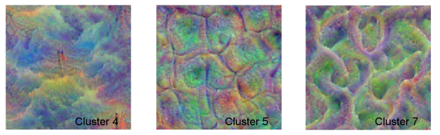
Cluster 4 clearly prefers smooth and cloudy inputs, whereas cluster 5 likes smaller tiles, separated by dark edges. However, it is difficult to say what the network makes out of those features. First, they will interact with other feature maps. Second, the Gram matrix analysis does not tell whether the feature map clusters are active at all for a given input, or at which locations. Second, as mentioned before, textures are not determined by patterns of feature activations, but by correlations of feature activations.

So let’s go one step further and modify the deep dream algorithm in order to maximize the correlational structure within a cluster of features in a layer, instead of the simple activations of the features. Here comes the result for cluster 4, with the deep dream maximizing either the activity in this cluster of features (left) or maximizing the correlational structure across features within in this cluster (right).

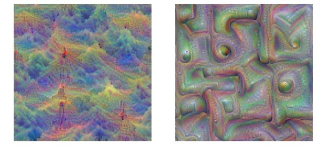
The result is, maybe surprisingly, little informative. It shows that the texture of clouds is not located in a single cluster of the Gram matrix (which is optimized for in the right-hand image), but distributed across the full spectrum of features, and probably also across several layers.

Together, the analysis so far has shown how Gram matrices look like, how they cluster and to how these clusters can be interpreted. However, the complexity and the distributed nature of computations in the network make it very difficult to intuitively understand what is going on and to predict what would happen to specific layers or feature maps or Gram matrices when exposed to a given input picture.

To sum it up, correlated features (= Gram matrices) can be used to compare the textures of two images and can be employed by a loss function to measure texture similarity. This works both for texture synthesis and style transfer. As a byproduct, the correlation matrix of feature maps, the Gram matrix, can be used to understand how the feature space is divided up by a bunch of clusters of similarly tuned channels. If you want to play around with this, my Jupyter notebook on Github could be a good starting point.

An interesting aspect is the fact that joint statistics – a somewhat arbitrary and empirical measurement – are sufficient to generate textures that seem natural to humans. Would it not be a good idea for the human brain, when it comes to texture instead of object recognition, to read out correlated activity of ‘feature neurons’ of the same receptive field and them simply average over all receptive fields? The target neurons that read out co-active feature neurons would thus see some the Gram matrix of the feature activations. There is already work in experimental and theoretical neuroscience that goes somewhat into this direction (Okazawa et al., 2014, link, short summary here).

For further reading, I can recommend Li et al., 2017 (link), who reframe the Gram matrix method by describing it as a Maximum Mean Discrepancy (MMD) minimization with a specific kernel. In addition, they show that other kernels are also useful to measure distances between feature distributions, thereby generalizing the style transfer method. (On the other hand, this paper did not really improve my intuitive understanding of style transfer.)
For an overview of implementations of the style transfer method, there is a nice and recent review on style transfer by Ying et al., 2017 (link). It is not really well-written, but very informative and concise.