With the experience of more than one year of patching (although you might say that this is not a lot), I’m now used to problems that I can solve after some time, but without being able to tell what the problem has been (neuronal health? osmolarity of the intracellular solution? pipette tip shape? … ?). Especially electrical noise is sometimes tricky to track down, and attempts to improve the noisiness often tend to be fruitless, or successful, but without a clear understanding what happend. See for example this anecdotal report on denoising a setup that starts with: “For three weeks I have been banging my head against the wall.”
Here, I would like to show one example where I was not only successful in removing a noise artifact, but could also understand it (to some extent). To put it in context, I had installed my electrophysiology rig, together with a system of grounding cables that worked perfectly in blocking any noise from micromanipulators or other components of the 2P microscope that I’m using for targeted shadow-patching. However, there was still a line-frequency component of 50 Hz (it’s Europe) that I could not understand or remove. It wasn’t there when I tried to debug it without a brain sample, but it was there when I started doing experiments.
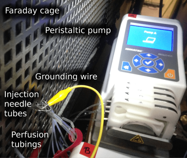
It turned out that the noise came from the perfusion system. I have a persistaltic pump (this one) that is located outside of the Faraday cage. It drives the ACSF perfusion of the brain under my microscope, and apparently the ACSF was transfering the 50 Hz signal from the pump directly to my preparation. This was tricky to understand, because when I used simple distilled water for water, it did not, because of its lower conductivity, transport the noise into the setup.
For a couple of days, I tried to somehow shield the pump from the perfusion system, but since the perfusion tubings and the peristaltic pumps are too tightly connected, I didn’t manage to. Finally it was an advice from my thesis supervisor (Rainer Friedrich) that solved the problem. He suggested to ‘ground’ the perfusion. It did not make so much sense to me (the ground electrode was already in the bath, why ground it again in the middle of the perfusion tubing?), but I did try it out. At the point where the perfusion tubing goes through the Faraday cage, I cut the tubing and inserted the stainless steel tubes taken from an injection needle, which in turn I connected to ground.
To cut the story short, it worked! It’s pretty much self-explanatory:
Recently, I mentioned a public competition for spike detection – spikefinder.codeneuro.org. I decided to spend a day two days and have a closer look at the datasets, especially the training datasets that provide both simultaneously recorded calcium and spike trains for single neurons. In the following paragraphs, I will try to convey my impression of the dataset, and I will show some home-brewed and crude, but nicely working attempts to infer spiking probabilities from calcium trains. [Update: Together with Stephan Gerhard, I’ve designed a better algorithm based on CNNs to infer spiking probabilities, described on this blog and on Github.]
The training dataset consists of 10 separate datasets, recorded in different brain regions and using different calcium indicators (both genetically encoded and synthetic ones), each dataset with 17±10 neurons, and each neuron recorded for several hundred seconds.
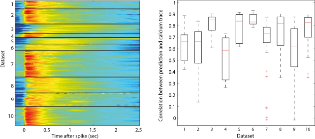
To check the quality of the recordings, I calculated the cross-correlation function between spike train and calcium trace to get the shape of the typical calcium event that follows a spike (it is kind of similar to a PSTH, but takes also cases into consideration where two spikes occur at the same time). I have plotted those correlation functions for the different datasets, one cross-correlation shape for each neurons (colormap below, left). Then I convolved the resulting shape with the ground truth spike train.
If calcium trace and spike train were consistent, the outcome of the convolution would be highly correlated with the measured calcium signal. This is indeed the case for some datasets (e.g. dataset 6; below, right). For others, some neurons show consistent behavior, whereas others don’t, indicating bad recording quality either of the calcium trace or the spike train (e.g. the low correlation data points in datasets 2, 4, 7 and 9).
In my opinion, those bad recordings should have been discarded, because there is probably no algorithm in the world that can use them to infer the underlying spike times. From looking at the data, I got the impression that it does not really make sense to try to deconvolve low-quality calcium imaging recordings as they are sometimes produced by large-scale calcium imaging.
But now I wanted to know: How difficult it is to infer the spike rates? I basically started with the raw calcium trace and tried several basic operations to find something that manages to come close to the ground truth. In the end, I used a form of derivative, by subtracting the calcium signal of a slightly later (delayed) timepoint from the original signal. I will link the detailed code below. I was surprised how little parameter tuning was required to get quite decent results for a given dataset. Here is the core code:
% calculate the difference/derivative
prediction = calcium_trace - circshift(calcium_trace,delay);
% re-align the prediction in time
prediction = circshift(prediction,-round(delay/2));
% simple thresholding cut-off
prediction( prediction < 0 ) = 0;
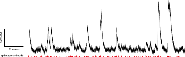
Let me show you a typical example of how the result looks like (arbitrary scaling):
Sometimes it looks better, sometimes worse, depending on data quality.
The only difficulty that I encountered was the choice of a single parameter, the delay of the subtracted calcium timetrace. I realized that the optimal delay was different for different datasets, probably due to different calcium indicator. Presumably, this reflects the fact that for instance calcium traces of synthetic dyes like OGB-1 (bright baseline, low dF/F) look very different from GCaMP6f traces (dim baseline, very high dF/F). Those properties can be disentangled e.g. by calculating the kurtosis of the calcium time trace.
Although this is based on only 10 datasets, and although I do not really know the reason why, the optimal delay in my algorithm seemed to depend on the kurtosis of the recording in a very simple way that could be fitted by a simple function (e.g. a double-exponential, or simply a smooth spline):
In the end, this algorithm is barely longer than 20 lines in Matlab (loading of the dataset included), in the simplicity spirit of the algorithm suggested by Dario Ringach. Here’s the full algorithm on Github. I will also submit the results to the Spikefinder competition in order to see how good this simple algorithm is compared to more difficult ones that are based on more complex models or analysis tools.
Close to my apartment in the outskirts of Basel, green fields and some small woods lie basically in front of my house door. This is also where some flocks of crows gather around, partly searching the fields for food, partly watching out in the topmost trees. Meeting them once every day, I started wondering whether these animals would qualify for being an animal model for neuroscience and especially neurophysiology.
Nowadays, mainstream neuroscience focuses on mice; next, on drosophila, zebrafish, C. elegans, some monkeys and the rat. Everything else (frog, honey bee, lizard, ferret …) is considered rather exotic – although there are millions of animal species on our planet, each of them with a different brain organization. Of course it does make sense to focus on a common species (that is ideally genetically tractable) as a community, in order to profit from synergies. But at the same time this narrows the mind. In my opinion, it is useful to have some researchers (although not the majority of them) work on exotic animal models – on those animals that stand out by a striking organization, by the simplicity of their brain, or by behaviors reminding of human behavior.
There is a long tradition, going back to John J. Audubon (*1785), Johann F. Naumann (*1780) and beyond of trying to embrace the world of birds by patient observation and detailed description. Until now, there is a large community of ‘birders’ who often content themselves with observing birds and the behaviors and features that help to identify a bird species. At some point – quite late, and probably later than for other animal species -, cognitive neuroscience questions that were targeted at birds came up: how intelligent are birds? do birds recognize themselves in mirrors? can birds count? what kind of language do they use? do birds form human-like families?
But is there any neurophysiological research on crows? What behaviors do they exhibit? Do they have brain structures homologues to the human brain? And, to start with, what are crows anyway, viewed in the context of the tree of life?
How are crows related to other species?
To visualize the phylogenetic tree of corvids in the context of other birds and standard neuroscience animal models, I used some information provided by the Tree Of Life project and put it together in a small drawing.
From this, it is clear that, for example, the ancestors of zebrafish branch very early from the human ancestors (430 ma, million years ago). Then reptiles including birds (312 ma), whereas mice are much closer to primates (90 ma). Drosophila and C. elegans (both almost 800 ma) are very far from all the vertebrates. In the bird family chicken and pigeons are very far from the songbirds, and given this broader context, corvids and other songbirds like zebra finches are phylogenetically close (44 ma, compared to ca. 82 million years between crows and falcons/pigeons/owls/parrots or 98 million years between crows and chicken). I looked up the times using www.timetree.org.
Of course this summary alone does not allow to perfectly choose an animal model. But it gives a first idea about the relationships. And I admit that I found it very instructive to make this drawing.
What kind of behaviors do crows show?
Crows do talk to each other using calls, by which they not only articulate their inner status, but also communicate information about the environment to others, e.g. about predators. A large variety of raven calls have been documented by Bernd Heinrich, Thomas Bugnyar and others (see e.g. [1]). However, calls are often locally or individually different, which makes the collection of a complete repertoire of calls impossible or at least meaningless.
Ravens are able to understand the capabilities and limitations of others, e.g. competitors [2]. To have an internal conception of the knowledge of specific others is an ability that might be related to the concept of empathy and therefore be an interesting field of study.
The smallest unit of corvid social life is the mating partnership, and crows usually choose their partner for a lifetime, but they also participate in larger social assemblies, e.g. for sharing information, sleeping and for hunting.
Similar to humans, and different from mice, crows rely mostly on visual and acoustic stimuli, rather than olfactory ones.
Crows are usually rather shy, but curious at the same time. The shyness is, of course, a problem for researchers wanting to work with crows. Especially wild crows are very difficult to tame, and it requires a lot of continuous work and personal care to raise a crow or a raven.
Bernd Heinrich tells about his rearing raven nestlings. He observes that curiosity and exploratory fearlessness dominates in the first months, after which shyness towards humans and a general extremely neophobic behavior dominates [3].
Unlike most other birds, crows are able to count [4]. For more context on the representations of numbers in crows, as compared to in primates, see [5].
At SfN 2016, I talked to some crow researchers (mainly working on memory tasks), and I was told that crows can often learn the same tasks as monkeys can, like a delayed choice task, on a very similar learning time scale.
Crows are well-known for their creativity (e.g. dropping walnuts on streets, where they are cracked by vehicles running over) and famous for using tools, especially the New Caledonian crow. Personally, I got the impression that crows plan ahead in time much more than any other birds – maybe this is also related to them being so shy.
Are there homologies between crow brains and human brains?
In a popular view held since the early 20th century, most of the avian telencephalon was seen as homologous to the striatum, which does not seem to play the central role for mammalian cognition. Around 2000, his theory was reversed by evidence from anatomy and genetic markers [6], now converging to the theory that a large fraction of the avian brain is actually of pallial and not striatal origin. The nuclei of which the avian telencephalon consists are supposed to be somewhat similar in connectivity to the layers of cortex.
The drawing below (modified from [7]) is a coronal section through the brain of a jungle crow, with the cutting position indicated on the left side (at least that’s my guess).
In an anatomical study done in chicken [8], local interlaminar recurrent circuits comparable to the laminar organization of mammalian cortex were found between the enteropallium (E in the schematic above, yellow) and the mesopallial ventro-lateral region (MVL, green), provided with input from thalamic structures (around ‘TFM’). This similarity to mammalian cortex organization is suggested to be due to convergent evolution, but not necessarily an organizational principle of a common ancestor. A short and readable, but very informative review of theories about homologies between bird and mammalian brains and convergent evolution has been put together by Onur Güntürkün [9], in whose lab also a first functional characterization of the – possibly associational – target areas of the enteropallium (NFL, MVL, TPO and NIL) is given by checking the expression of the immediate early gene ZENK [10].
What physiological methods are established for use with crows?
Not in crows, but in zebra finch, calcium imaging and optogenetic experiments [11] have been performed. The crow brain, however, is ca. 2 cm in size and therefore too big for invasive methods based on scattering light. I would guess that calcium imaging with virally expressed or synthetic calcium dyes would still be feasible on the brain surface. However, the avian brain probably does not expose its interesting ‘cortical’ structures at the outer surface, as do mammalian brains. Plus, an interesting brain structure, the nidopallium caudolaterale (NCL, [12]), which is supposed to work on similar tasks as the mammalian prefrontal cortex, is nicely accessible in pigeons, but located at the difficult-to-access lateral side of the brain in crows. Probably ultrasound-based methods that have been developed for rats [13] for coarse level activity imaging would be a good compromise, although they do not go down to cellular resolution.
Despite the challenges, the NCL is one of the corvid brain regions that has been recorded from [12], with 8 chronically implanted microelectrodes recording simultaneously in a delayed response behavioral task (similar to the classic experiments developed for prefrontal cortex in monkeys), where neurons firing in the waiting period of the behavioral task seem to encode an abstract rule that is lateron used for decision.
Other neurophysiological methods applied to crows include functional imaging using fMRI and the previously mentioned study using expression levels of the immediate early gene ZENK in order to find out tuning to motion or color [10], but all of this is clearly at very early and exploratory stages.
Further reading about crows and videos about crows.
This is an excellent basic FAQ on daily life interactions with crows, written by an academic researcher. .
A well-written book by raven behavior researcher Bernd Heinrich: Mind of the Raven, basically consisting of a large and sometimes a bit lengthy set of anecdotal stories. He writes among others about the struggles of raising raven nestlings and about the difficulties of mating them. .
An amateur crow researcher describing his crows and their typical behavior (video 18:15 min, german). .
Conclusion.
In my eyes, the corvid family is a very interesting animal model, since corvids show complex behavior like planning, creativity, tool-use and the ability to fly. On the other hand, they are more difficult to keep and raise than mice (which can simply be ordered for a couple of bucks). Their shyness is also a problem – try to approach a crow in the field, and you will know that it is not easy (although there are some exceptional, more curious crow individuals).
Realistically, I do not expect crows to become one of the major animal models – technique-wise, the field is simply too much behind the mouse- or monkey-field. But crow research might offer an important differing view on the brain. Probably some, even higher-order computations in crows and primates are very similar, and it would be interesting to see whether their implementations on a neuronal level are also similar and have developed in a convergent manner.
———————-
Bugnyar, Thomas, Maartje Kijne, and Kurt Kotrschal. “Food calling in ravens: are yells referential signals?” Animal Behaviour 61.5 (2001): 949-958. (link)
Bugnyar, Thomas, and Bernd Heinrich. “Ravens, Corvus corax, differentiate between knowledgeable and ignorant competitors.” Proceedings of the Royal Society of London B: Biological Sciences 272.1573 (2005): 1641-1646. (link)
Heinrich, Bernd, and Hainer Kober. Mind of the raven: investigations and adventures with wolf-birds. New York: Cliff Street Books, 1999. (link)
Ditz, Helen M., and Andreas Nieder. “Numerosity representations in crows obey the Weber–Fechner law.” Proc. R. Soc. B. Vol. 283. No. 1827. The Royal Society, 2016. (link)
Nieder, Andreas. “The neuronal code for number.” Nature Reviews Neuroscience (2016). (link)
Jarvis, Erich D., et al. “Avian brains and a new understanding of vertebrate brain evolution.” Nature Reviews Neuroscience 6.2 (2005): 151-159. (link with paywall)
Izawa, Ei-Ichi, and Shigeru Watanabe. “A stereotaxic atlas of the brain of the jungle crow (Corvus macrorhynchos).” Integration of comparative neuroanatomy and cognition (2007): 215-273. (link)
Ahumada‐Galleguillos, Patricio, et al. “Anatomical organization of the visual dorsal ventricular ridge in the chick (Gallus gallus): layers and columns in the avian pallium.” Journal of Comparative Neurology 523.17 (2015): 2618-2636. (link)
Güntürkün, Onur, and Thomas Bugnyar. “Cognition without cortex.” Trends in cognitive sciences 20.4 (2016): 291-303. (link)
Stacho, Martin, et al. “Functional organization of telencephalic visual association fields in pigeons.” Behavioural brain research 303 (2016): 93-102. (link)
Roberts, Todd F., et al. “Motor circuits are required to encode a sensory model for imitative learning.” Nature neuroscience 15.10 (2012): 1454-1459. (link with paywall)
Veit, Lena, and Andreas Nieder. “Abstract rule neurons in the endbrain support intelligent behaviour in corvid songbirds.” Nature communications 4 (2013). (link)
Macé, Emilie, et al. “Functional ultrasound imaging of the brain.” Nature methods 8.8 (2011): 662-664. (link)
Photos/Pictures/Videos:
Alpine cough (Alpendohle) on Mt. Pilatus/Switzerland, Summer 2016.
Raven soaring on Hawk Hill next to San Francisco, Fall 2016.
The main drawback of functional calcium imaging is its slow dynamics. This is not only due to limited frame rates, but also due to calcium dynamics, which are a slow transient readout of fast spiking activity.
A perfect algorithm would infer the spike times of each neuron from the calcium imaging traces. Despite ongoing effort for more than 10 years, no such algorithm is around – as most inverse problems, this one is a hard one, suffering from noise and variability. Then, it is difficult to generate ground truth (electrophysiological attached-cell recording of an intact cell and simultaneous calcium imaging). Plus, algorithms working for one dataset do not easily generalize to others.
To make comparison between algorithms easier, a competition was set up, based on several ground truth datasets from four different labs. If you are using an algorithm for deconvolution, test it out on their data. The datasets are easy to load in Matlab and Python (the spike train/calcium trace above is taken from one of the datasets) and are interesting by themselves even independent of this competition. Please check out the website of Spikefinder.
If I understand it correctly, it is mostly managed by Philipp Berens (Tuebingen/Germany) and Jeremy Freeman (Janelia/US).
I hope this competition will get a lot of attention and will make different algorithms easier to compare!
P.S. This competition made me also aware of another one going on earlier this year, which was less about spike finding, and more about cell identification and segmentation for calcium imaging data (Neurofinder).
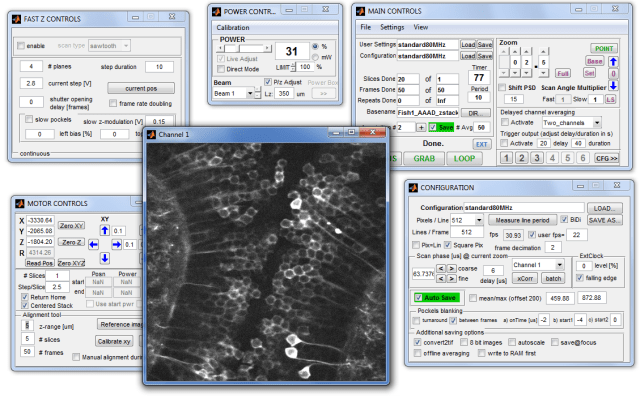
For control of resonant scanning 2P microscopes, my host lab uses a software that I have written in Matlab. Due to some coincidences, the software is based on Scanimage 4.2, a version developed few years ago for an interface with a Thorlabs scope and Thorlabs software (DLLs). I basically threw out the whole Thorlabs software parts, rewrote the core processing code, but kept the program structure and the look-and-feel (see a screenshot below: looks like Scanimage, but it isn’t). For anybody interested, I uploaded the code to Github on my Instrument Control repository. The program’s name is scanimageB, to make clear that it is based on scanimage, but different at the same time.
As hardware, the system is based on an Alazar 9440 DAQ board for 80 MHz acquisition with 2+ channels, where I was inspired by Dario Ringach’s Scanbox blog. Everything apart from acquisition is done using NI DAQ 6321 boards as in the original scanimage 4.2. Those boards are the cheapest X series DAQ boards. Some more details on the design are in this paper.
The software does not aim to be any kind of competitor for scanimage, scanbox, helioscan, sciScan, MScan or others. I do not even want other labto use this software for their microscopes. Instead, I’m hoping that people will find code snippets in the repository that might be useful for their own projects.
The code is not fully self-explanatory, and some core features (data acquisition) are partly dependent on the Alazar source developmental kit (ATS-SDK), which is cheap, but not open software. But if you are interested in a specific microscope control problem, send me a message, so that I can point you to the relevant code snippet which I used to solve this particular problem. Just let me know below in the comments or via eMail —
Here are some of the more interesting sections of the software:
MEX/C-code that uses native windows threads in C for parallelization and speeding up processing inside of Matlab. I use it to convert the 80 million data points per second per channel into pictures of arbitrary binning. Most other 2P resonant scanning microscopes do this task on (expensive) FPGAs. .
In one of the main m-files, search for scanphaseAdjust(obj). This is an algorithm that I’m using for automated scan phase adjustment for bidirectional scanning. The implementation is not designed for speed, but it features sub-pixel precision alignment by very simple means. .
In another big Matlab file which I repurposed from something written by Thorlabs, you can find how I implemented the integration of the Alazar 9440 DAQ board into Matlab using Alazar’s SDK, e.g. in the function PRinitializeAlazar(obj). When I started, I did not find any Matlab code online for controling this board, so this might serve as a starting point for other people as well. .
If you want to use retriggerable tasks for X-Series NI DAQ boards, you can search for the key words Task( and retriggerable in this code. Retriggerable tasks are important to understand if you want to synchronize devices on a sub-microsecond timescale using NI DAQ boards. This code snippets will give you a good idea how this can be done using the open DABS library (a Matlab instrument control library written by the Scanimage programmers). It works basically as in Labview, but the code can be understood more easily afterwards and by others.
Precise synchronization and reliable fast triggering is – in my opinion – the most challenging part of writing a control software for resonant scanning microscopes. To this end, I’m using the internal memory of the programmable X series NI DAQ boards to overcome these fast timescales (thereby following Scanimage 4.2 and 5.0). But the complex interdependence of triggers for laser pulses, lines, frames, laser shutters and pockels cells, together with the synchronization of external hardware makes things complicated and difficult to debug. If you are facing similar challenges of implementing complex triggering tasks, I would be glad to point you to sample code or give you some hopefully helpful advice —
A couple of days ago, I discovered a list of neuroblog feeds managed by Neurocritic, covering almost 200 blogs in total. Out of those, I picked the blogs most relevant for circuit and cellular neuroscience. This excludes most blogs on cognitive neuroscience and fMRI studies, and also those that focus on reproducibility and publishing issues or on science career advice rather than science itself. I preferred blogs which are well-written and still active, and which cover more than the papers of the lab or person that is running the blog. I also included blogs that focus on techniques and neuroengineering (those are covered here).
I put letters in front to inform about some of the blogs’ contents: is a blog run by a neuroscience lab. discusses scientific papers (though not always in depth). includes some focus on computational aspects of neuroscience. And openly discusses not only research papers and technical stuff, but also big questions that a general public might find intriguing.
Neuwritewest is an ambitious project aiming at making neuroscience more accessible to a broader public. It features paper presentations, and interviews with renown neuroscientists (‘Neurotalk’): http://www.neuwritewest.org/
Lists of recent papers on computational neuroscience and related topics. Including discussion of big questions in neuroscience, by Romain Brette: http://romainbrette.fr
Critical and very detailed discussion of recent neuroscience papers, by Markus Meister: https://markusmeister.com/
From the lab of Anne Churchland from CSHL. Good discussion of recent topics in neuroscience and journal club discussions of single papers: https://churchlandlab.org/
A blog by neuroscientist Anita Devineni about her work experience with fruit flies and about big questions and topics in neuroscience. The blog is nicely designed and very well written: http://www.brains-explained.com
A blog dedicated to bringing up and sometimes also discussing paper (mainly preprints posted on ArXiv and bioRxiv), run by the Steve Shea from CSHL: https://idealobserverblog.wordpress.com/
A blog discussing important papers with a focus on the hippocampus, run by Jake Jordan, a neuroscience PhD student in NY: https://nervoustalk.wordpress.com/
In a recent blog post about deep learning based on raw audio waveforms, I showed what effect a naive linear dynamic range compression from 16 bit (65536 possible values) to 8 bit (256 possible values) has on audio quality: Overall perceived quality is low, mostly because silence and quiet parts of the audio signal will get squished. The Wavenet network by Deepmind, however, uses a non-linear compression of the audio amplitude that allowed to map the signal to 8 bit without major losses. In the next few lines, I will describe what this non-linear compression is, and how well it performs on real music.
For two-photon point scanning microscopy, the excitation laser is typically pulsing at a repetition rate of 80 MHz, that is one pulse each 12.5 ns. To avoid aliasing, it was suggested to synchronize the sampling clock to laser pulses. For this, it is important to know over how much time the signal is smeared, that is, to measure the duration of the transient.
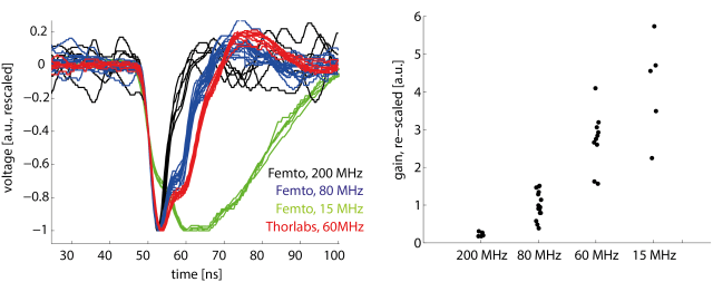
The device that smooths the PMT signal over time is the current-to-voltage amplifier. As far as I know, the two most commonly used ones are the Femto DHPCA-100 (variable gain, although mostly used with the 80 MHz bandwidth setting) and the Thorlabs model (60 MHz fixed bandwidth).
Observing single transients for different preamplifiers
However, 80 MHz bandwidth does not mean that everything below 80 MHz is transmitted and everything beyond suppressed. The companies provied frequency response curves, but in order to get a better feeling, I measured the transients of the above-mentioned preamplifiers when they amplified a single photon detected by a PMT. All transients are rescaled in y-direction (left-hand plot). I also determined a sort of gain for the single events by measuring the amplitude (right-hand plot). I also used two preamplifiers for each model, but could not make out any performance difference between two of the same kind.
For the 80 MHz bandwidth setting (Femto), the transient does not fully decay even after 15 ns or later; the Thorlabs preamp is even slower than this. Both exhibit a smooth multi-step shape during the decay phase.
At first glance, the Thorlabs preamp seems to be the obvious best choice, since the bandwidth is similar to the Femto 80 MHz and the gain is 3x higher. But for functional imaging, electrical noise is not a big problem, since the main source of noise is simply photon shot noise. In my hands, neither of both clearly outperformed the other, although this might be different for a completely different set of PMT/fluorophor/SNR.
The 200 MHz Femto setting would be perfect for lock-in sampling (and I already used it for that purpose), but the gain is, at least for my PMT, at the limit where electrical noise can become dominant (see figure on the right side). The 15 MHz setting, on the other hand, does not give any advantage, except if one samples with much less than 80 MHz.
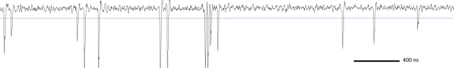
Counting photons using an oscilloscope vs. using Poisson statistics
Looking at the raw oscilloscope traces when the microscope is scanning a biological sample, one can make another interesting observation. Shown here is a time window spanning 4000 ns, that is, 320 laser pulses. But those laser pulses only manage to elicit 14 photon-detecting events.
As many neuroscientists, I’m also interested in artificial neural networks and am curious about deep learning networks. I want to dedicate some blog posts to this topic, in order to 1) approach deep learning from the stupid neuroscientist’s perspective and 2) to get a feeling of what deep networks can and can not do. Part I, Part II, Part III, Part IVb.
One of the most fascinating outcomes of the deep networks has been the ability of the deep networks to create ‘sensory’ input based on internal representations of learnt concepts. (I’ve written about this topic before.) I was wondering why nobody tried to transfer the deep dreams concept from image creation to audio hallucinations. Sure, there are some efforts (e.g. this python project; the Google project Magenta, based on Tensorflow and also on Github; or these LSTM blues networks from 2002). But to my knowledge no one had really tried to apply convolutional deep networks on raw music data.
Therefore I downsampled my classical piano library (44 kHz) by a factor of 7 in time (still good enough to preserve the musical structure) and cut it into some 10’000 fragments of 10 sec, which yields musical pieces each with 63’000 data points – this is slightly fewer datapoints than are contained by 256^2 px images, which are commonly used as training material for deep convolutional networks. So I thought this could work as well. However, I did not manage to make my deep convolutional network classify any of my data (e.g., to decide whether a sample was Schubert or Bach), nor did the network manage to dream creatively of music. As most often with deep learning, I did not know the reasons why my network failed.
Now, Google Deepmind has published a paper that is focusing on a text-to-speech system based on a deep learning architecture. But it can also be trained using music samples, in order to lateron make the system ‘dream’ of music. In the deepmind blog entry you can listen to some 10 sec examples (scroll down to the bottom).
As key to their project, they used not only convolutional filters, but so-called dilated convolutions, thereby being able to span more length-(that is: time-)scales with fewer layers – this really makes sense to me and explains to some extent why I did not get anything with my normal 1d convolutions. (Other reasons why Deepmind’s net performs much better include more computational power, feedforward shortcut connections, non-linear mapping of the 16bit-resolved audio to 8bit for training and possibly other things.)
The authors also mention that it is important to generate the text/music sequence point by point using a causal cut-off for the convolutional filter. This is intuitively less clear to me. I would have expected that musical structure at a certain point in time could very well be determined also by future musical sequences. But who knows what happens in these complex networks and how convergence to a solution looks like.
Another remarkable point is the short memory of the musical hallucinations linked above. After 1-3 seconds, a musical idea is faded because of the exponential decaying memory; a bigger structure is therefore missing. This can very likely be solved by using networks with dilated convolutions that span 10-100x longer timescales and by subsampling the input data (they apparently did not do it for their model, probably because they wanted to generate naturalistic speech, and not long-term musical structure). With increasing computational power, these problems should be overcome soon. Putting all this together, it seems very likely that in 10 years you can feed the full Bach piano recordings into a deep network, and it will start composing like Bach afterwards, probably better than any human. Or, similar to algorithms for paintings, it will be possible to input a piano piece written by Bach and let a network which has learned different musical styles continuously transform it into Jazz.
On a different note, I was not really surprised to see some sort of convolutional networks excel at hallucinating musical structure (since convolutional filters are designed to interpret structure), but I am surprised to see that they seem to outperform recurrent networks for generation of natural language (this comparison is made in Deepmind’s paper). Long short-term memory recurrent networks (LSTM RNNs, described e.g. on Colah’s blog, invented by Hochreiter & Schmidhuber in ’97) solve the problem of fast-forgetting that is immanent to regular recurrent neuronal networks. I find it a bit disappointing that these problems can also be overcome by blown-up dilated convolutional feed-forward networks, instead of neuron-intrinsic (more or less) intelligent memory in a recurrent network like in LSTMs. The reason for my disappointment is due the fact that recurrent networks seem to be more abundant in biological brains (although this is not 100% certain), and I would like to see research in machine learning and neuronal networks also focus on those networks. But let’s see what happens next.
Ever since I my interested in neuroscience become more serious, I was fascinated by the patch clamp technique, especially applied for the whole cell. Calcium imaging or multi-channel electrophysiology (recent review) is the way to go in order to get an idea what a neuronal population is doing on the single-cell level, but it occludes fast dynamics like bursting, fast oscillations and subthreshold membrane potential dynamics (calcium imaging), or unambiguous assignment of activity to single neurons (multi-channel ephys). That’s exactly what whole-cell patch clamp can do (and much more).
Some months ago, I started using the technique on an adult zebrafish brain ex vivo preparation. This image shows a z-stack of a patched cell that was imaged after the electrical recording. The surrounding cells are labeled with GCaMP; the brighter labeling of the patched neuron was done by a fluorophor inside the pipette that was diffusing into the cell, with which the pipette ideally forms a single electrical compartment. The fluorophor fills up the soma and some of the dendrites. The pipette position is shown as an overlay in the right-hand side image.
Electrophysiology is a very unrewarding and difficult activity, compared to calcium imaging. The typical, old-school electrophysiologist is always alone with his rig, through long nights of a never-ending series of failures, intercepted by few successfully patched and nicely behaving neurons. On average, frustration dominates, no matter how successful he/she is in the end; as a consequence, he fiercely protects his rig from anybody else who wants to touch it and might interfere with the labile stability of his setup. Therefore, over time, he becomes more and more annoyed by any interaction with fellow humans. At least that is what people say about electrophysiologists …
Despite this asocial component, nothing is more encouraging for beginners like me than hearing from others and about their struggles with electrophysiology. I will therefore write about my own experience with electrophysiology so far, and although I’m lacking the year-long experience of older electrophysiologist, I share my experience with the hope to encourage others.
To begin with, here’s a list of useful books and manuals for learning, if one does not have an experienced colleague who shows every single detail:
Areles Molleman, Patch Clamping: An Introductory Guide to Patch Clamp Electrophysiology
A very short book which does not go into the details e.g. of analog electrical circuits of a cell, but gives useful pragmatic advice and how-to-dos for patching (both single channel and whole-cell). Very useful starting point for the beginner. .
In Labtimes, there’s a 2009 short first-hand report [the website is no longer online, but you can access it with the waybackmachine link] by Steven Buckingham that highlights some of the difficulties of patching and gives precise and concise advice. .
The Axon Guide for Electrophysiology & Biophysics Laboratory Techniques
If you have time for 250 pages of technical descriptions, this is your choice. The document might be quite old, but there haven’t been many revolutions to patching anyway. For several troubleshooting issues, I have found good advice in this document. .
If you are lacking the theoretical background of how neurons, membrane potentials and ions work together, I would recommend online lectures like these slides that have a focus on theoretical underpinnings of measurements and not on measurements and troubleshooting. .
For a more in-depth description of everything related to membrane potentials and ions: Ion Channels of Excitable Membranes (3rd Ed.) by Bertil Hille. It’s 15 years old, but still the best book that I’ve seen so far. Especially for somebody with a physics background, it is very rewarding to read. .
For questions related to applications of patching (and other single neuron-specific tools), I can recommend Dendrites by Stuart, Spruston, Häusser et al., although I have not yet checked the newest, very recent edition (2016)..


![Brain of a jungle crow in relation to its head. Coronal slice at the location that I indicated on the left side (my guess). The fibers between E (Entopallium) and MVL are sort of sensory pathways coming from thalamus (via TFM). Both pictures modified from [6].](https://gcamp6f.com/wp-content/uploads/2016/11/crowbrain.jpg?w=597&h=401)
 As hardware, the system is based on an Alazar 9440 DAQ board for 80 MHz acquisition with 2+ channels, where I was inspired by Dario Ringach’s Scanbox blog. Everything apart from acquisition is done using NI DAQ 6321 boards as in the original scanimage 4.2. Those boards are the cheapest X series DAQ boards. Some more details on the design are in this
  is a blog run by a neuroscience lab.
  discusses scientific papers (though not always in depth).
  includes some focus on computational aspects of neuroscience. And
  openly discusses not only research papers and technical stuff, but also big questions that a general public might find intriguing.