For two-photon point scanning microscopy, the excitation laser is typically pulsing at a repetition rate of 80 MHz, that is one pulse each 12.5 ns. To avoid aliasing, it was suggested to synchronize the sampling clock to laser pulses. For this, it is important to know over how much time the signal is smeared, that is, to measure the duration of the transient.

The device that smooths the PMT signal over time is the current-to-voltage amplifier. As far as I know, the two most commonly used ones are the Femto DHPCA-100 (variable gain, although mostly used with the 80 MHz bandwidth setting) and the Thorlabs model (60 MHz fixed bandwidth).

Observing single transients for different preamplifiers

However, 80 MHz bandwidth does not mean that everything below 80 MHz is transmitted and everything beyond suppressed. The companies provied frequency response curves, but in order to get a better feeling, I measured the transients of the above-mentioned preamplifiers when they amplified a single photon detected by a PMT. All transients are rescaled in y-direction (left-hand plot). I also determined a sort of gain for the single events by measuring the amplitude (right-hand plot). I also used two preamplifiers for each model, but could not make out any performance difference between two of the same kind.

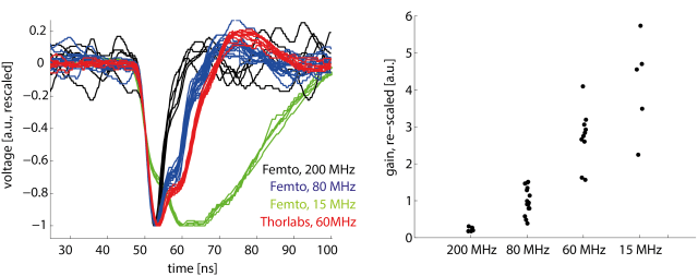
For the 80 MHz bandwidth setting (Femto), the transient does not fully decay even after 15 ns or later; the Thorlabs preamp is even slower than this. Both exhibit a smooth multi-step shape during the decay phase.

At first glance, the Thorlabs preamp seems to be the obvious best choice, since the bandwidth is similar to the Femto 80 MHz and the gain is 3x higher. But for functional imaging, electrical noise is not a big problem, since the main source of noise is simply photon shot noise. In my hands, neither of both clearly outperformed the other, although this might be different for a completely different set of PMT/fluorophor/SNR.

The 200 MHz Femto setting would be perfect for lock-in sampling (and I already used it for that purpose), but the gain is, at least for my PMT, at the limit where electrical noise can become dominant (see figure on the right side). The 15 MHz setting, on the other hand, does not give any advantage, except if one samples with much less than 80 MHz.

Counting photons using an oscilloscope vs. using Poisson statistics

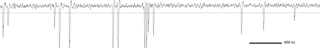
Looking at the raw oscilloscope traces when the microscope is scanning a biological sample, one can make another interesting observation. Shown here is a time window spanning 4000 ns, that is, 320 laser pulses. But those laser pulses only manage to elicit 14 photon-detecting events.

Let’s put this into some context. Normally, I bin every 8 laser pulses to one pixel; therefore, counting the detected photons per 8 pulses gives the photons per pixel. The outcome of doing this for each oscilloscope trace gives a couple of numbers (# photons per pixel bin), which are plotted below as single data points and histogram (figure to the right). Here, the number of photons per pixel bin is between 0.1 and 0.9 photons. In other words, only every 10-50th laser pulse creates a fluorescence photon that is detected lateron.

For the same sample, I also recorded an image and determined the number of photons per pixel as described earlier (based on a Labrigger blog post). As far as I can tell from the small statistics for photon counting using oscilloscope traces, there is a surprisingly close agreement between the two independent measurements. It might be off by a factor 1.5 or less.

On a side note, the reason for the low number of photons compared to this earlier example is a different fluorophor. In the previously shown example, it was the artificial calcium sensor rhod-2 which features a high baseline fluorescence; here, the tissue is weakly labeled with GCaMP6f, which has a much lower baseline fluorescence (actually, the tissue shown here is actually probably dead and therefore a little bit brighter than normal GCaMP6f-labeled neurons).

What I learned from this:

1. Neither the Femto DHCP-100 at 80 MHz nor the Thorlabs preamplifier are very well-suited for lock-in sampling to 80 MHz laser pulses.
   .
2. For normal samples (by which I mean: functional calcium imaging), despite a difference in gain (factor 3), both preamps perform similarly, since for both the signal is stronger than electrical noise.
   .
3. Normally, I (and certainly others with dim samples) get < 1 photon per pixel for GCaMP, and << 1 photon per laser pulse. Given by how many infrared photons the tissue is hit (around 10^9 photons per pulse!), this is astounding.
   .
4. Calculating the gain of the system and the number of photons per pixel using the method mentioned before yields results that are consistent with (oscilloscope) photon counting. It appears as if one really can rely on this easy method to estimate the number of photons per pixel. This can be an important piece of information when one needs to decide whether to implement a photon counting hardware solution for a given applicatoin or not.

Update [ 2016-09-22 ] :

Upon Dario’s comment, I looked into what happens if you sample at 80 MHz (i.e., synced to the laser pulses), but at different phase lags, as described on the Scanbox blog by Tobias Rose. Using the transients measured above, one can simulate the phase-dependence of the signal intensity. The intensity ratio of best timing vs. worst timing is around 3 for the Femto 80 MHz, and <2 for the Thorlabs 60 MHz. This means that the sampling phase relative to the laser pulses is definitely important, and more for the Femto preamp than for the Thorlabs one. (I do not see this strong dependence with my microscope, but this may be due to a badly behaving laser sync signal.)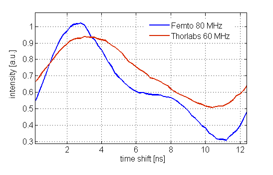

To make things more complicated, this factor of up to 3 means a threefold increase in signal, but not a threefold increase in SNR. SNR is mainly determined by shot noise, not voltage amplitude; however, I would bet that electrical noise can become quite prominent in the trough of the phase plot, and phase optimization still increases SNR.