In a recent blog post about deep learning based on raw audio waveforms, I showed what effect a naive linear dynamic range compression from 16 bit (65536 possible values) to 8 bit (256 possible values) has on audio quality: Overall perceived quality is low, mostly because silence and quiet parts of the audio signal will get squished. The Wavenet network by Deepmind, however, uses a non-linear compression of the audio amplitude that allowed to map the signal to 8 bit without major losses. In the next few lines, I will describe what this non-linear compression is, and how well it performs on real music.

Nonlinear dynamic range compression

A quick search shows that the compression scheme used by the Wavenet is far from original, having been installed as an international standard for communication (although there are actually two standards, the European A-law standard and the US µ-law standard). The transformations, here the µ-law for 8 bit,

are more or less logarithmic, which corresponds roughly to the psychophysics of human perception. To be precise, the subjective loudness of audio stimuli rather follows a power law than a logarithmic expression, but this is only important for the limit regimes (high and low frequencies).

A second possibility of compression that one could think of for reducing audio file size (in order to generate compact training data for machine learning) is the method used for mp3s and similar formats. It is called MDCT (modified discrete cosine transform) and is basically a derivative of a discrete Fourier transform (DFT). The output of the transform therefore lives in Fourier/frequency space. Deep learning based on such datasets could still be efficient. But then there would be no real need for convolutional filters, since time as a variable is already eliminated by the MDCT. Also, operating in the frequency instead of the time domain would be less intuitive for exploration. Which is a disadvantage: In my opinion not only the output of a network is important, but also the ease of understanding what happens inside the network during learning and recall.

Minimal dynamic bit depth for J.S. Bach

To examine the performance of the non-linear compression, I will use a real (piano music) example to showcase the effects of linear/non-linear dynamic compression. As a test sample, here is a rather calm intro to a piece by J.S. Bach. First the original, 16 bit:

Next follows the naive, linearly compressed dynamic range (8 bit) version. Brace yourself for some unpleasant noise:

However, if the signal is compressed non-linearly via the µ-law algorithm to 8 bit as described above (I tried the A-law as well: little difference; I slightly preferred the µ-law):

This sounds much better, despite some remaining whispering in the background. Not bad! But are all of those 8 bit really required? Why not reduce it to, e.g., 4 bit dynamic range? To test this, I resampled the excerpt at a bit depth that is increasing over time, starting with 4 bit (everything below is rather painful).

The change in bitdepth over time is plotted below. Even in the raw signal, the reduced bitdepth can be seen from the coarsely discretized amplitude values at the beginning – at 4 bit, the volume can take only 2^4 = 16 different values. This is clearly not good enough for human ears.

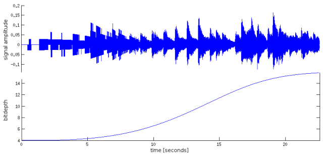
With 6 bits, it starts sounding better, and is almost fully re-covered at a bit depth of 11-12 (this depends on the quality of your earphones – with standard loudspeakers, I would guess that 8-9 bits might already sound the same as the original). However, the decisive quality increase seems to happen between 6 and 8 bit. Let’s make a fairer comparison.

5 bit (which sounds like footsteps in the snow …): 

6 bit:

7 bit:

My conclusion: If I wanted to create a dataset with piano music for deep learning, I would go for 6-7 bit dynamic range. 5-6 bit seems to be too low quality to me. The reduction from 8 to 6-7 bit seems to be small, but it reduces the possible values from 256 to ca 100. This can be important for an implementation like Wavenet, where these 256 or 100 values are discrete categories upon which the input of the network is mapped. Leaving the network with too many category choices, it is probably much easier to make it fail with a given task.

P.S. Matlab script

For completeness, here is a small Matlab script that reads in an mp3, reduces the bit depth according to the µ-law and writes it to a sound file (*.wav). If you comment the blue lines, you will get the naive linear 8 bit compression variant and a lot of noise.

% read audio file
[audioX,sampling_rate] = audioread('JSBach.mp3');
% transform
bitdepth = 8;
audioX = sign(audioX).*log(1+(2^bitdepth-1).*abs(audioX))./log(2^bitdepth);
% discretize to 8 bit
audioX = double(round(audioX*(2^(bitdepth-1))))/(2^(bitdepth-1));
% transform back to normal
audioX = sign(audioX).*((2^bitdepth).^abs(audioX) - 1)./(2^bitdepth - 1);
% play 8 bit audio
soundsc(audioX,Fs);
% save audio back to file
audiowrite('JSBach_mod.wav',audioX,Fs);

Newer versions of Matlab (which I do not have) already have implemented the compression algorithm in the function compand(). In Python, the audioop library will help you out.