Preamplifier bandwidth & two ways of counting photons

For two-photon point scanning microscopy, the excitation laser is typically pulsing at a repetition rate of 80 MHz, that is one pulse each 12.5 ns. To avoid aliasing, it was suggested to synchronize the sampling clock to laser pulses. For this, it is important to know over how much time the signal is smeared, that is, to measure the duration of the transient.

The device that smooths the PMT signal over time is the current-to-voltage amplifier. As far as I know, the two most commonly used ones are the Femto DHPCA-100 (variable gain, although mostly used with the 80 MHz bandwidth setting) and the Thorlabs model (60 MHz fixed bandwidth).

Observing single transients for different preamplifiers

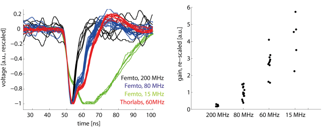
However, 80 MHz bandwidth does not mean that everything below 80 MHz is transmitted and everything beyond suppressed. The companies provied frequency response curves, but in order to get a better feeling, I measured the transients of the above-mentioned preamplifiers when they amplified a single photon detected by a PMT. All transients are rescaled in y-direction (left-hand plot). I also determined a sort of gain for the single events by measuring the amplitude (right-hand plot). I also used two preamplifiers for each model, but could not make out any performance difference between two of the same kind.

preamps.png

For the 80 MHz bandwidth setting (Femto), the transient does not fully decay even after 15 ns or later; the Thorlabs preamp is even slower than this. Both exhibit a smooth multi-step shape during the decay phase.

At first glance, the Thorlabs preamp seems to be the obvious best choice, since the bandwidth is similar to the Femto 80 MHz and the gain is 3x higher. But for functional imaging, electrical noise is not a big problem, since the main source of noise is simply photon shot noise. In my hands, neither of both clearly outperformed the other, although this might be different for a completely different set of PMT/fluorophor/SNR.

The 200 MHz Femto setting would be perfect for lock-in sampling (and I already used it for that purpose), but the gain is, at least for my PMT, at the limit where electrical noise can become dominant (see figure on the right side). The 15 MHz setting, on the other hand, does not give any advantage, except if one samples with much less than 80 MHz.

Counting photons using an oscilloscope vs. using Poisson statistics

Looking at the raw oscilloscope traces when the microscope is scanning a biological sample, one can make another interesting observation. Shown here is a time window spanning 4000 ns, that is, 320 laser pulses. But those laser pulses only manage to elicit 14 photon-detecting events.

traces

Continue reading

Posted in Calcium Imaging, Imaging, Microscopy | Tagged , , , | 10 Comments

Deep learning, part IV: Deep dreams of music, based on dilated causal convolutions

As many neuroscientists, I’m also interested in artificial neural networks and am curious about deep learning networks. I want to dedicate some blog posts to this topic, in order to 1) approach deep learning from the stupid neuroscientist’s perspective and 2) to get a feeling of what deep networks can and can not do. Part I, Part II, Part III, Part IVb.

One of the most fascinating outcomes of the deep networks has been the ability of the deep networks to create ‘sensory’ input based on internal representations of learnt concepts. (I’ve written about this topic before.) I was wondering why nobody tried to transfer the deep dreams concept from image creation to audio hallucinations. Sure, there are some efforts (e.g. this python project; the Google project Magenta, based on Tensorflow and also on Github; or these LSTM blues networks from 2002). But to my knowledge no one had really tried to apply convolutional deep networks on raw music data.

Therefore I downsampled my classical piano library (44 kHz) by a factor of 7 in time (still good enough to preserve the musical structure) and cut it into some 10’000 fragments of 10 sec, which yields musical pieces each with 63’000 data points – this is slightly fewer datapoints than are contained by 256^2 px images, which are commonly used as training material for deep convolutional networks. So I thought this could work as well. However, I did not manage to make my deep convolutional network classify any of my data (e.g., to decide whether a sample was Schubert or Bach), nor did the network manage to dream creatively of music. As most often with deep learning, I did not know the reasons why my network failed.

Now, Google Deepmind has published a paper that is focusing on a text-to-speech system based on a deep learning architecture. But it can also be trained using music samples, in order to lateron make the system ‘dream’ of music. In the deepmind blog entry you can listen to some 10 sec examples (scroll down to the bottom).

As key to their project, they used not only convolutional filters, but so-called dilated convolutions, thereby being able to span more length-(that is: time-)scales with fewer layers – this really makes sense to me and explains to some extent why I did not get anything with my normal 1d convolutions. (Other reasons why Deepmind’s net performs much better include more computational power, feedforward shortcut connections, non-linear mapping of the 16bit-resolved audio to 8bit for training and possibly other things.)

The authors also mention that it is important to generate the text/music sequence point by point using a causal cut-off for the convolutional filter. This is intuitively less clear to me. I would have expected that musical structure at a certain point in time could very well be determined also by future musical sequences. But who knows what happens in these complex networks and how convergence to a solution looks like.

Another remarkable point is the short memory of the musical hallucinations linked above. After 1-3 seconds, a musical idea is faded because of the exponential decaying memory; a bigger structure is therefore missing. This can very likely be solved by using networks with dilated convolutions that span 10-100x longer timescales and by subsampling the input data (they apparently did not do it for their model, probably because they wanted to generate naturalistic speech, and not long-term musical structure). With increasing computational power, these problems should be overcome soon. Putting all this together, it seems very likely that in 10 years you can feed the full Bach piano recordings into a deep network, and it will start composing like Bach afterwards, probably better than any human. Or, similar to algorithms for paintings, it will be possible to input a piano piece written by Bach and let a network which has learned different musical styles continuously transform it into Jazz.

On a different note, I was not really surprised to see some sort of convolutional networks excel at hallucinating musical structure (since convolutional filters are designed to interpret structure), but I am surprised to see that they seem to outperform recurrent networks for generation of natural language (this comparison is made in Deepmind’s paper). Long short-term memory recurrent networks (LSTM RNNs, described e.g. on Colah’s blog, invented by Hochreiter & Schmidhuber in ’97) solve the problem of fast-forgetting that is immanent to regular recurrent neuronal networks. I find it a bit disappointing that these problems can also be overcome by blown-up dilated convolutional feed-forward networks, instead of neuron-intrinsic (more or less) intelligent memory in a recurrent network like in LSTMs. The reason for my disappointment is due the fact that recurrent networks seem to be more abundant in biological brains (although this is not 100% certain), and I would like to see research in machine learning and neuronal networks also focus on those networks. But let’s see what happens next.

Continue reading

Posted in machine learning | Tagged , , , | 8 Comments

Whole-cell patch clamp, part 1: introductory reading

Ever since I my interested in neuroscience become more serious, I was fascinated by the patch clamp technique, especially applied for the whole cell. Calcium imaging or multi-channel electrophysiology (recent review) is the way to go in order to get an idea what a neuronal population is doing on the single-cell level, but it occludes fast dynamics like bursting, fast oscillations and subthreshold membrane potential dynamics (calcium imaging), or unambiguous assignment of activity to single neurons (multi-channel ephys). That’s exactly what whole-cell patch clamp can do (and much more).

Some months ago, I started using the technique on an adult zebrafish brain ex vivo preparation. This image shows a z-stack of a patched cell that was imaged after the electrical recording. The surrounding cells are labeled with GCaMP; the brighter labeling of the patched neuron was done by a fluorophor inside the pipette that was diffusing into the cell, with which the pipette ideally forms a single electrical compartment. The fluorophor fills up the soma and some of the dendrites. The pipette position is shown as an overlay in the right-hand side image.

Electrophysiology is a very unrewarding and difficult activity, compared to calcium imaging. The typical, old-school electrophysiologist is always alone with his rig, through long nights of a never-ending series of failures, intercepted by few successfully patched and nicely behaving neurons. On average, frustration dominates, no matter how successful he/she is in the end; as a consequence, he fiercely protects his rig from anybody else who wants to touch it and might interfere with the labile stability of his setup. Therefore, over time, he becomes more and more annoyed by any interaction with fellow humans. At least that is what people say about electrophysiologists …

Despite this asocial component, nothing is more encouraging for beginners like me than hearing from others and about their struggles with electrophysiology. I will therefore write about my own experience with electrophysiology so far, and although I’m lacking the year-long experience of older electrophysiologist, I share my experience with the hope to encourage others.

To begin with, here’s a list of useful books and manuals for learning, if one does not have an experienced colleague who shows every single detail:

  • Areles Molleman, Patch Clamping: An Introductory Guide to Patch Clamp Electrophysiology
    A very short book which does not go into the details e.g. of analog electrical circuits of a cell, but gives useful pragmatic advice and how-to-dos for patching (both single channel and whole-cell). Very useful starting point for the beginner.
    .
  • In Labtimes, there’s a 2009 short first-hand report [the website is no longer online, but you can access it with the waybackmachine link] by Steven Buckingham that highlights some of the difficulties of patching and gives precise and concise advice.
    .
  • The Axon Guide for Electrophysiology & Biophysics Laboratory Techniques
    If you have time for 250 pages of technical descriptions, this is your choice. The document might be quite old, but there haven’t been many revolutions to patching anyway. For several troubleshooting issues, I have found good advice in this document.
    .
  • If you are lacking the theoretical background of how neurons, membrane potentials and ions work together, I would recommend online lectures like these slides that have a focus on theoretical underpinnings of measurements and not on measurements and troubleshooting.
    .
  • For a more in-depth description of everything related to membrane potentials and ions: Ion Channels of Excitable Membranes (3rd Ed.) by Bertil Hille. It’s 15 years old, but still the best book that I’ve seen so far. Especially for somebody with a physics background, it is very rewarding to read.
    .
  • For questions related to applications of patching (and other single neuron-specific tools), I can recommend Dendrites  by Stuart, Spruston, Häusser et al., although I have not yet checked the newest, very recent edition (2016)..

Soon, I hope that I will have time to write about some more technical aspects of patching. (Here about how to remove line-frequency noise that stems from the perfusion pump, about the limitations of quantitative whole cell voltage-clamp recordings, especially in small neurons, about blue light-induced artifacts in whole-cell recordings, and about the look and feel of two-photon targeted patching, including several instructive movies.)

Posted in electrophysiology, Microscopy, zebrafish | Tagged , , , | 2 Comments

The larval zebrafish, and the adult zebrafish

Zebrafish are often used as a model organism for in vivo brain imaging, because they are transparent. Or at least that is what many people think who do not work with zebrafish. In reality, most people use zebrafish larvae for in vivo imaging, typically not older than 5 days (post fertilization). At this developmental stage, the total larval body length is still less than the brain size of the adult fish. After 3-4 weeks, the fish look less like tadpoles and more like fish, measuring 10-15 mm in size (see also video below). They attain the full body length of approx. 25 to 45 mm within 3-4 months.

This video shows a zebrafish larva (7 days old), two adult zebrafish (16 months old) and a juvenile zebrafish (4.5 weeks old).

.
After 4-5 days, the brain size of larvae exceeds the dimensions that can be imaged with cellular resolution in vivo using light sheet or confocal microscopy when embedded in agarose. After approx. 4 weeks, even for unpigmented fish the thickened skull makes imaging of deeper brain regions very difficult. Superficial brain regions like the tectum are better accessible, but fish of this age are too strong to be restrained by agarose embedding. Brain imaging for adult fish is still possible in ex vivo whole brain preparations [1], but with loss of behavioral readout. Use of toxins for immobilization is an option (e.g. with curare in zebrafish [2] or in other fish species [3]), but not a legal one in some countries, including Switzerland. These are some of the reasons why most people stick to the simple zebrafish larva. My PhD lab is one of the few that does physiology in adult zebrafish.

Posted in Calcium Imaging, Neuronal activity, zebrafish | Tagged , | Leave a comment

Neuroscience on Youtube

Recently, I’ve been to the Basel ICON conference, where the recent Nobel laureate Eric Betzig gave an impressive talk on microscopy techniques (including lattice light sheet, SIM and expansion microscopy). Some days ago, I found a similar talk by Eric Betzig (although with less recent results) simply on youtube.
The advantages of online videos compared to live talks are obvious, and I wonder why people do not use them more often, both to learn about research and to communicate their own research. Additionally, compared to research papers, the personality of a researcher is much more obvious from a talk – which is important to know for students interested in working in his/her lab. Here just a small collection of some good talks by neuroscientists which are not as flashy and fancy as TED talks, but much more informative and interesting.

Here is Eve Marder on central pattern generators in lobsters and crabs. She had been developing experiments and models for this seemingly simply system for more than 40 years, thereby exposing the complexity of a system consisting of only 30 neurons.

Ken Harris, a mathematician by training and now more interested in large-scale brain activity recordings in mice, gives a rather technical, but very understandable talk on advances and problems in spike sorting for multielectrode arrays.

Larry Abbott, one of the most well-known theoreticians in neuroscience, with a very interesting talk about experimental findings in the olfactory system of the fruit fly.

Christof Koch on the search for the neuronal correlates of consciousness. In the late 90s, he was one of the pioneers in this field together with Francis Crick; more recently, he is working together with Giulio Tononi.

Edvard Moser on spatial navigation and place cells/grid cells. For this topic he was awarded the Nobel prize 2014.

Haim Sompolinsky with a theoretical perspective on sensory representations memory in distributed circuits. Coming from physics, Haim Sompolinsky helped transferring the physics of phase transitions to the mathematical modeling of neuronal network models in the late 80s.

Some of the links might be outdated in a couple of years, but I hope that researchers will start uploading more recent and well-prepared talks in the years to come, replacing overcrowded plenary talks by often jet-lagged speakers.

Update [2016-07-20]: Maybe this is the right place to mention a very nice series of podcasts, featuring interviews with leading neuroscientists, e.g. Michael Shadlen or Peter Jonas, or of my thesis supervisor in Basel, Rainer Friedrich. Thanks to Anne Urai who posted a link to this webpage on her blog.

Posted in Data analysis, Microscopy, Network analysis | Tagged , | Leave a comment

Large field of view microscopes for mouse brain imaging

For typical confocal or two-photon microscopes that maintain (sub)cellular resolution, a high-magnification objective is needed (typically 16x, 20x or 25x). This in turn limits the field of view (FOV) to ⌀ 1.0-1.5 mm.

For imaging in the mouse brain cortex, which is basically a big unwrinkled surface of a size of the order of 10 mm, a bigger FOV would be nice to have for some applications. Recently, a couple of papers came out that tried to increase the FOV, while using optical engineering to maintain the resolution. (Please don’t hesitate to tell me if I missed a relevant publication.)

Few years ago, I would have expected such papers to be published in Nature Methods, but apparently the time has come where optical engineering and improvement of existing techniques is not considered enough for passing the novelty bar. However, the three papers offer some very interesting lessons on engineering a two-photon microscope, of which I want to pick a few:

Continue reading

Posted in Calcium Imaging, Imaging, Microscopy | Tagged , , | 7 Comments

Spatial visualization of temporal components for neuronal activity imaging

The standard analysis workflow for neuronal activity imaging based on calcium signals is to 1) draw ROIs around putative neurons, 2) extract the average fluorescence time trace of this ROI, 3) work with this timetrace for subsequent analysis (principal components, correlations between neuronal timetraces, tuning, etc).

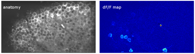
For spatial visualization, typically a dF/F map is used, based on a F0 image and a time window used for computation of the dF map, showing the neurons active during a given time window. Here an example for one plane of the movie shown in a previous blog post.

anatomy_dF

I have rarely seen people mapping more complex temporal components back to space, although this is really easy … here I want to give an example, which I have used in a very similar way to create Fig.5D in this paper. (I have mentioned this paper earlier on this blog.) Here, I want to apply it to one plane of a small-volume recording.

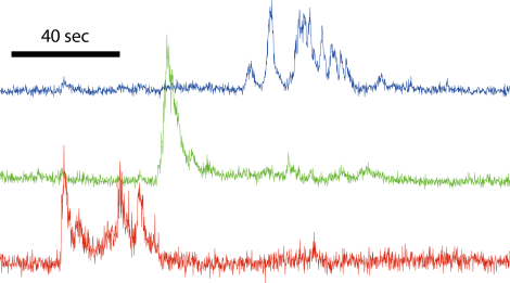
First, I use the timecourses of single neuronal soma ROIs to calculate the temporal principal components of the time course of this set of neurons; or, often better, to generate clusters and the mean timetrace of each cluster. Here are the first three temporal clusters, showing three different dynamic features:

Traces

Next, I go back to the raw data and check each pixel for the correlation of the pixel’s time course with the time course of the components shown above. This gives one value for each pixel, i.e., in total a correlation map. This representation maps the temporal component back to space for all the three principal components that I’ve shown above. Here, the left picture corresponds to the red trace, the center picture to the green trace, the right picutre to the blue trace above.

RGB_gray

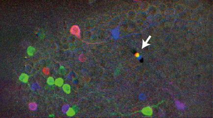
It is possible to condense this representation even further, by mapping each of the three spatial maps to one of the Red/Green/Blue color channels. In total, this is a spatial color-mapping of temporal components back to anatomy. I won’t discuss the biological interpretations here, but I find this data representation both appealing (although I’m partially colorblind) and helpful for understanding spatial structures.

RGB

Although being partially colorblind, I really like this color-coded spatial map. The arrow points to an artifact not related to neuronal activity, but a blood cell moving through a blood vessel during imaging.

The Matlab code behind this spatial mapping is very simple. Assuming you have the raw data (“movie”) and three extracted components (“clusters”):

movie; % 3D raw data, NxMxT (width x height x timepoints)
clusters; % extracted components TxW (T = timepoints, W = [1,2,3])

% 1 = R, 2 = G, 3 = B
for k = 1:3
   xcorr_tot = zeros(size(movie,1),size(movie,2));
   for j = 1:size(movie,1)
      xcorr_tot(j,:) = corr(clusters(:,k),squeeze(movie(j,:,:))');
   end
   RGB_map{k} = xcorr_tot;
end
Posted in Calcium Imaging, Data analysis, Imaging, Neuronal activity | Tagged , | Leave a comment

Reglo ICC serial port control via Matlab

For my experiments with zebrafish, I typically generate dynamic odor landscapes for the fish / fish brain explant by varying the speed of the wheels of an Ismatec peristaltic pump, thereby changing the concentration of the applied stimuli over time. Recently, I bought one of their digital pumps (Reglo ICC with four independent channels), but the company only provides a Labview code sample for custom implementation.

I wrote a small Matlab adapter class to interface with the pump. In order to spare other people from this effort, here is my implementation on Github. It allows to change pump speed, pumping direction etc by a serial protocol that is transmitted via USB and a virtual COM port. – It should be easy to use this as a starting point for a similar code snippet in Python.

Clearly, this will be useful for only a small number of people, but I at least would have been glad to find a sample code in the internet that could have spared me the time to write the code by myself. Hopefully Google will find its way to direct people in need to these links. Here are some guiding tags: Reglo ICC, Ismatec, Cole-Parmer, serial port, USB, COM, serial object, adapter class, object-oriented Matlab.

Posted in Uncategorized | Tagged , , , , , | 13 Comments

Fast z-scanning using a voice coil motor

We just published a paper on fast remote z-scanning using a voice coil motor. For 2P calcium imaging. It’s a nice paper with some interesting technical details.

The starting point was the remote z-scanning scheme used by Botcherby et al. (2012) from Tony Wilson’s lab, but we modified the setup to make it easier to implement for an existing standard 2P microscope, and we used only off-the-shelf components, for in total <2500 Eur.

The first challenge when implementing the Tony Wilson remote scanning scheme was to find something that can move a mirror in axial direction with high speed (sawtooth, >5 Hz). Botcherby et al. used a costum-built system consisting of a metal band glued to synchronized galvos. In order to simplify things (for details on optics etc, see the paper), I was looking for a device that comes off-the-shelf and that can move fast in a linear way over a couple of millimeters. That is, a very fast linear motor. Typical linear motors are way too slow (think of a typical slow microscope stage motor).

End of 2014, I found a candidate for such a linear motor: loudspeakers. When you have a close look at large subwoofers, you can see that the membranes move over many millimeters in extreme cases; and such loudspeakers are used for operation between 20 Hz and 10 kHz, so they are definitely fast. So I bought a simple loudspeaker for 8 Euro and glued a mirror onto the membrane. However, precision in the very low frequency domain (< 50 Hz) was limited, at least for the model I had bought:

loudspeaker

But as you can see, this is a very simple device: A permanent magnet and two voltage input pins, nothing else. Ok, there is the coil that is attached to the backside of the membrane, but it remains very simple. The copper coil is permeated by magnetic field and therefore experiences a force when electrical current flows through the coil, thereby inducing motion of the coil and the attached membrane.

In spring 2015, I realized that the working principle of such loudspeakers is called “moving coil” or ” voice coil”, and using this search term I found some suppliers of voice coil motors for industrial applications. These applications range from high repeatability positioning devices (such as old-fashioned, non-SSD hard drives) to linear motors working at >1000 Hz with high force to mill a metal surface very smoothly.

So, after digging through some company websites, I bought such a voice coil motor together with a servo driver and tried out the wiring, the control and so on. It turned out to be such a robust device that it is almost impossible to destroy it. I was delighted to see this, since I knew how sensitive piezos can be e.g. when you push or pull into a direction that does not convene to the growth direction of the piezo crystal.

This is how the voice coil motor movement looks like in reality inside of the setup. I didn’t want to disassemble the setup, so it is here within the microscope. To make the movements visible for the eye, it is scanning very slowly (3 Hz). On top of the voice coil motor, I’ve glued the position hall sensor (ca. 100 Euro). I actually used tape and wires to fix the positions sensor – low-tech for high-precision results.

The large movement of the attached mirror is de-magnified to small movements of the focus in the sample, thereby reducing any positional noise of the voice coil motor. This is also the reason why I didn’t care so much about fixing the hall sensor in a more professional way.

After realizing that it is possible to control the voice coil motor with the desired precision, repeatability and speed, it remained to consider more closely the optics of the remote scanning system. Actually, more than two third of the time that I spent for this paper were related to linear ABCD optics calculations, PSF measurements and other tests of several different optical configurations, rather than being related to the voice coil motor itself.

More generally, I think that voice coil motors could be interesting devices for a lot of positioning tasks in microscopy. The only problem: To my knowledge, typical providers of voice coil motors have rather industrial applications in mind, which reduces the accessibility of the technique for a normal research lab. A big producer of voice coil motors is SMAC, but they seem to have customers that want to buy some thousand pieces for an industrial assembly line. I prefered both the customer support and the website of Geeplus and I bought my voice coil motor from this company – my recommendation.
As described in the paper, I used an externally attached simple position sensor system, but there are voice coil motor systems that have an integrated encoder. Companies that sell such integrated systems are Akribis Systems and Equipsolution, and our lab plans to have a try with those (mainly because of curiosity). Those solutions use optical position sensors with encoders instead of a mechanical hall sensors, increasing precision and lowering the moving mass, but also at higher cost.
One problem with some of these companies is that they are – different from Thorlabs or similar providers – not targeted towards researchers, and I found it sometimes difficult or impossible to get the information I needed (e.g. step response time etc.). If I were to go for a voice coil motor project without previous experience, I would either go the hard way and just buy one motor plus driver that look fine (together, this can easily be <1000 Euro, that is, not much) and try out; or stick to the solution I provided in the paper and use it as a starting point; or ask an electrical engineer who knows his job to look through some data sheets and select the voice coil motor that you want to have for you. I did it the hard way, and it worked out for me in a very short time. Me = physics degree, but not so much into electronics. I hope this encourages others to try out similar projects themselves!

During the review process of the paper, one of the reviewers pointed out a small recent paper that actually uses a regular loudspeaker for a similar task (field shaping). This task required only smaller linear movements, but it’s still interesting to see that the original idea of using a loudspeaker can somehow work.

Since then, I’ve been using the voice coil motor routinely for 3D calcium imaging in adult zebrafish. Here is just a random example of a very small volume, somewhere in a GCamped brain, responding to odor stimuli. Five 512 x 256 planes scanned at 10 Hz. The movie is not raw data, but smoothed in time. The movies selected for the paper are of course nicer, and the paper is also open access, so check it out.


Posted in Calcium Imaging, Imaging, Microscopy, Neuronal activity | Tagged , , , | 3 Comments

Modulating laser intensity on multiple timescales (x, y and z)

In point-scanning microscopy and especially when using resonant scanners, the intensity of the beam is typically modulated using a Pockels cell. For resonant scanning, the dwell time per micrometer is not constant along the scanned line, and one wants either to modulate the laser intensity accordingly (here’s an example) or at least shut down the laser beam at the turnaround points, where the velocity of the scanner is basically zero for some microseconds. A command signal to shut down the laser for this period could look similar to this one on a noise oscilloscope, with the dips representing the laser beam blanking during the turnaround points:

LineDip

However, sometimes the tissue is illuminated inhomogeneously, and it would be nice to increase the laser power when scanning the dim parts of the FOV. For example, in the adult zebrafish brain that I’m working with, the bottom of the FOV can be at the bright surface of the tissue, whereas the top of the image is dim due to its depth below some scattering layers of gray matter. In order to compensate for this inhomogeneity, I wanted to be able to modulate the pockels cell both in x, y, and at the turnarounds (x-direction). The problem is purely technical: In order to create a driving signal for the pockels cell on these two timescales (less than microseconds and more than milliseconds), one needs high temporal resolution and a long signal ( a long “waveform” in LabView speak). However, a typical NI DAQ board’s onboard memory is limited to 8192 data points. Which makes it impossible to modulate intensity in x and y.

I used a very simple solution to work around this problem. The idea is to generate two separate signals for modulation in x and y and then simply add the two output voltages. This does not allow for arbitrary 2D modulation patterns, but typically I’m happy with a linear combination of x- and y-modulation.
This solution disregards the non-linearity of a typical sine-shaped pockels cell calibration (input voltage vs. output laser intensity), but as long as the result is better than before, why not do it? This is what comes out:

ModulationExample

Note that the timescale is 25 microseconds on the left-hand side, and 25 milliseconds on the right-hand side.

The only technical challenge that I had to deal with was the following: From the DAQ boards, I get two separate voltage outputs. How do I sum them up? Of course, one can buy an expensive device that can do this and many other things by default. Or, one can build a summing amplifier, for less than 10 Euro:

summingAmplifier

Here is a description of this very simple circuit. Just use three equal resistors (labeled green), and you have an (inverting) unity gain voltage summer. In order to maintain the temporal precision, use a MHz operational amplifier (labeled red above). I bought this one for < 1 Euro. It took me less than 30 min with a soldering gun to assemble the summing amplifier, so it’s pretty easy. That’s how it looks like in reality, with an additional zoom-in of the core circuit:

summingAmp

And here is a small random brain region expressing GCaMP before (left) and after (right) the additional modulation in x and y:

BrainBoth

The average power is the same. The closer I looked, the more substantial the difference got. For example, the bright dura cells on the left are really annoying due to their brightness, but less so in the right-hand side image. I was surprised myself by how much this small feature improves imaging in curved brain regions, given the little money and effort it demanded.

Also, it is apparently straightforward to extend the y-direction modulation into a modulation in y and z, since the two timescales are similar (30-60 Hz framerate vs. 5-15 Hz volume rate for my experiments).

Posted in Calcium Imaging, Imaging, Microscopy | Tagged , , , | 1 Comment