The standard analysis workflow for neuronal activity imaging based on calcium signals is to 1) draw ROIs around putative neurons, 2) extract the average fluorescence time trace of this ROI, 3) work with this timetrace for subsequent analysis (principal components, correlations between neuronal timetraces, tuning, etc).

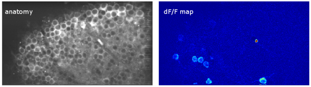
For spatial visualization, typically a dF/F map is used, based on a F0 image and a time window used for computation of the dF map, showing the neurons active during a given time window. Here an example for one plane of the movie shown in a previous blog post.

I have rarely seen people mapping more complex temporal components back to space, although this is really easy … here I want to give an example, which I have used in a very similar way to create Fig.5D in this paper. (I have mentioned this paper earlier on this blog.) Here, I want to apply it to one plane of a small-volume recording.

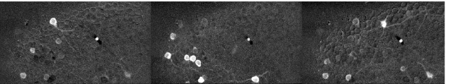
First, I use the timecourses of single neuronal soma ROIs to calculate the temporal principal components of the time course of this set of neurons; or, often better, to generate clusters and the mean timetrace of each cluster. Here are the first three temporal clusters, showing three different dynamic features:

Next, I go back to the raw data and check each pixel for the correlation of the pixel’s time course with the time course of the components shown above. This gives one value for each pixel, i.e., in total a correlation map. This representation maps the temporal component back to space for all the three principal components that I’ve shown above. Here, the left picture corresponds to the red trace, the center picture to the green trace, the right picutre to the blue trace above.

It is possible to condense this representation even further, by mapping each of the three spatial maps to one of the Red/Green/Blue color channels. In total, this is a spatial color-mapping of temporal components back to anatomy. I won’t discuss the biological interpretations here, but I find this data representation both appealing (although I’m partially colorblind) and helpful for understanding spatial structures.

Although being partially colorblind, I really like this color-coded spatial map. The arrow points to an artifact not related to neuronal activity, but a blood cell moving through a blood vessel during imaging.

The Matlab code behind this spatial mapping is very simple. Assuming you have the raw data (“movie”) and three extracted components (“clusters”):

movie; % 3D raw data, NxMxT (width x height x timepoints)
clusters; % extracted components TxW (T = timepoints, W = [1,2,3])

% 1 = R, 2 = G, 3 = B
for k = 1:3
   xcorr_tot = zeros(size(movie,1),size(movie,2));
   for j = 1:size(movie,1)
      xcorr_tot(j,:) = corr(clusters(:,k),squeeze(movie(j,:,:))');
   end
   RGB_map{k} = xcorr_tot;
end