Deep learning, part III: understanding the black box

As many neuroscientists, I’m also interested in artificial neural networks and am curious about deep learning networks. I want to dedicate some blog posts to this topic, in order to 1) approach deep learning from the stupid neuroscientist’s perspective and 2) to get a feeling of what deep networks can and can not do. Part I, Part IIPart IV, Part IVb. [Also check out this blog post on feature visualization; and I can recommend this review article.]

The main asset of deep convolutional neural networks (CNNs) is their performance; their main disadvantage is that they can be used with profit, but not really understood. Even very basic questions like ‘why do we use rectified linear units (RELUs) as activation functions instead of slightly smoothed versions?’ are not really understood. Additionally, after learning the network is a black box that performs exceedingly well, but one cannot see why. Or, it performs badly, and also to sometimes cryptic reasons. What has the network learned actually?

But there are some approaches that shed light on what has been learnt be CNNs. For example, there is a paper by Matthew Zeiler. I’ve mentioned a Youtube-Video by him in a previous post (link to video). He uses a de-convolution (so to say, a reverse convolution) algorithm to infer the preferred activation pattern of ‘neurons’ somewhere in the network. For neurons of the first layer, he sees very simple patterns (e.g. edges), with the patterns getting more complex for intermediate (e.g. spirals) and higher layers (e.g. dog face). The parallels to the ventral visual stream in higher mammals is quite obvious.

Google DeepDream goes into the same direction, but yielding more fascinating pictures. Basically, the researchers took single ‘neurons’ (or a set of neurons encoding e.g. animals) in the network and used a search algorithm to find images that activate this ‘neuron’ most. The search algorithm can use random noise as a starting point, or an image provided by the user. Finally, this leads to the beautiful pictures that are well-known by now (link to some beautiful images). Google has also released the source code, but within the framework of Caffè (link), and not Tensorflow. However, at the bottom line of this website, they promise to provide a version for Tensorflow soon as well [Update October 2016: It has been released now].

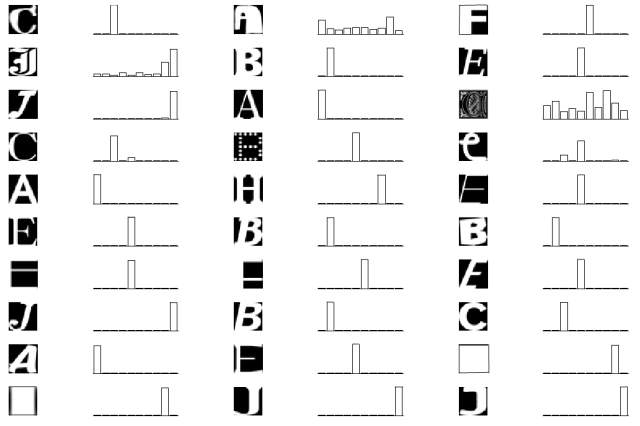
In the meantime, let’s have a less elaborate, but more naïve look, in order to get a better understanding of deep networks. I will try to dissect parts of a 5-layer convolutional network that I wrote during the Tensorflow Udacity course mentioned previously in this blog. For training, it uses a MNIST-like data, but a little bit more difficult. The task is to assign a 28×28 px image to one of the letters A-J. Here you can see how the network performs for some random test data. In the bar plot, the positions 1-10 correspond to the letters A-J, visualizing the certainty of the network.

fig1

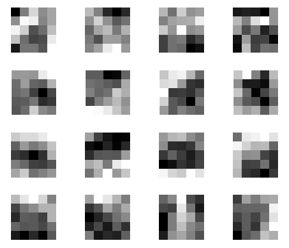
So let’s look inside the black box. The first layer in this network consists of sixteen 5×5 convolutional filters. Those filters had been established during learning. Here they are:

fig2

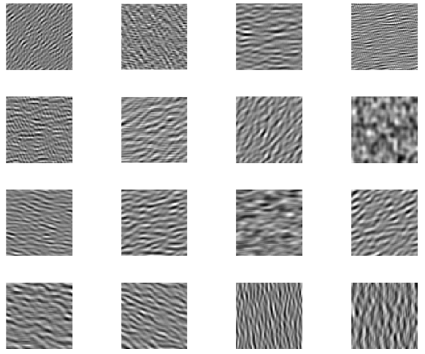
Does this make sense to you? If not, here are the 16 filters (repeatedly) applied to noise, revealing the structures that are made to detect:

fig3

Obviously, most of those filters have a preference for some (curved) edge elements (which is not really surprising).

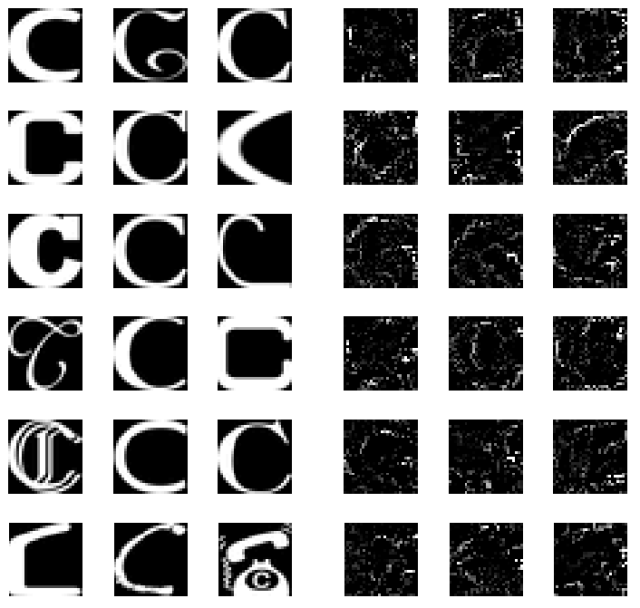
For simple networks like this one, which is not very deep and only has to learn simple letters, intermediate layers do not really represent something fancy (like spirals, stars or eyes). But one can at least have a look at how the ‘representation’ of the fifth layer, the output layer looks like. For example, what is the preferred input pattern of the output ‘neuron’ that has learned to assign the letter ‘C’?

To find this out, I used the same deep learning network as before, but kept constant the network weights that had been learnt before. Instead, I varied the input image, whilst telling the stochastic gradient descent optimizer to maximize the output of the ‘C’ neuron.

Starting from random noise, different local optimization maxima are reached, each of them corresponding more or less to an ‘idea of C’ that the deep network has in mind. The left side shows ‘C’s from the original dataset. The right hand side shows ideas of ‘C’ that I extracted from the network with my (crude) search algorithm. One obvious observation is that the extracted ‘C’s do not care about surfaces, but rather about edges, which can be expected from a convolutional network and from the filters of the first layer shown above.

fig4

Posted in machine learning | Tagged , , | 4 Comments

Undistort/unwarp images for resonant scanning microscopy

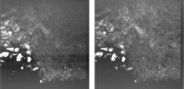
For image acquisition using a resonant scanning microscope, one of the image axes is scanned non-linearly, following the natural sinusoidal movements of the resonant scanner. This leads to a distortion of the acquired images, unless a online correction algorithm or temporal non-homogeneous sampling rate is used. A typical (averaged) picture:

unnormal

Clearly, the left and right side of the picture are streched out. This does not worry me if I only want to extract fluoresence time courses of neuronal ROIs; but it is a problem for nice-looking pictures that want to have a valid scalebar. Unfortunately, I didn’t find any script in the internet on how un-distorting is normally being done for resonant scanning, so I want to present my own (Matlab) solution for other people looking around. It is not elegant, but it works. For the final solution, scroll to the bottom of the blog entry.

Continue reading

Posted in Calcium Imaging, Microscopy | Tagged , , , , | 1 Comment

Deep learning, part II : frameworks & software

As many neuroscientists, I’m also interested in artificial neural networks and am curious about deep learning networks. I want to dedicate some blog posts to this topic, in order to 1) approach deep learning from the stupid neuroscientist’s perspective and 2) to get a feeling of what deep networks can and can not do. Part IPart IIIPart IV, Part IVb.

To work with deep learning networks, one can either write ones’s own functions and libraries for loss functions or backpropagation; or use one of the available “frameworks” that provide the libraries and everything else under the hood that is more interesting for developers, but not for users of deep learning networks.
Here’s a best of: Tensorflow, Theano, Torch, Caffe. Out of those, I would recommend either Tensorflow, the software developed and used by Google, and Theano, which is similar, but developed by academic researchers. Both can be imported as libraries in Python.

First, I tried to install both Theano and Tensorflow on Windows 7, and gave up after a while – both frameworks are not designed to work best on Windows, although there are solutions that do work (update early 2017: Tensorflow is now also available for Windows, although you have to take care to install the correct python version). So I switched to Linux (Mint) and installed Tensorflow, and spent some time digging out my Python knowledge that got lost during the last couple of years when I used Matlab only.

Here’s the recipe that should give a good handle on Tensorflow in 2-4 days:

  1. Installation of Tensorflow. As always with Python, this can easily take more than one hour. I installed a CPU-only version, since my GPU is not very powerful.
    .
  2. Some basic information to read – most of this applies to Theano as well.
    .
  3. Then here’s a nice MNIST tutorial using Tensorflow. MNIST is a standard number recognition dataset that is used as a standard benchmark for supervised classifiers.
    .
  4. For a more systematic introduction, check out the Tensorflow udacity class that has been announced recently on Google’s research blog, based on a dataset similar to MNIST, but a little bit more difficult to classify. The lecture videos are short and focused on a pragmatic understanding of the software and of deep learning. For deeper understanding, please read a book.
    .
    The core of the Tensorflow class is the hands-on part which consists of code notebooks that are made available on github (notebooks 1-4). This allows to understand the Tensorflow syntax and solve some “problems” by modifying small parts of the given sample code. This is really helpful, because googling for possible solutions to problems gives a broader overview of Tensorflow. Going through these exercises will take 1-3 days of work, depending on whether you are a perfectionist or not.
    .
  5. Now you should be prepared to use convolutions, max pooling, dropout and stochastic gradient descent on your own data with Tensorflow. I will try do to this in the next couple of weeks and report it here.

Here are some observations that I made when trying out Tensorflow:

  1. There are a lot of hyperparameters (learning rate, number of layers, size of layers, scaling factor of L2 regularization of different layers, shape/stride/depth of convolutional filters) that have to be optimized. Sometimes the behavior is unexpected or even unstable. I didn’t find good and reliable advice on how to set the hyperparameters in function of the classification task.
    .
  2. To illustrate the unpredictable behavior, here is a very small parameter study on a neural network (no convolutional layer) with two hidden layers with 50 and 25 units each. The factors L1 and L2 give the scaling of the L2 regularization loss term (for explanation see chapter 7.1.1 in this book) of the respective layers. If the loss function for the (smaller) second hidden layer is weighted more strongly than the loss function for the first hidden layer (i.e., L2 >> L1), the system is likely to become unstable and to settle to random assignment of the ten available categories (= 10% success rate). However, whether this happens or not depends also on the learning rate – and even on the initialization of the network.
    .

    L1\L2 1e-4 5e-4 1e-3 5e-3
    1e-4  89.9%  10.0%  10.0%  10.0%
    5e-4  91.8%  91.9%  92.1%  10.0%
    1e-3  92.3%  92.6%  92.2%  10.0%
    5e-3  10.0%  10.0% 89.3%  10.0%

    .

  3. When following the tutorial and the course, there is not much to be done except for tweaking algorithms and hyperparameters, with the only network performance readout being “89.1%”, “91.0%”,”95.2%”,”10.0%”,”88.5%” and so on; or maybe a learning curve. It’s a black box with some tunable knobs. But what has happened to the network? How did it learn? How does its internal representation look like? In one of the following weeks, I will have a look into that.
Posted in machine learning | Tagged , | 3 Comments

Deep learning, part I


As many neuroscientists, I’m also interested in artificial neural networks and am curious about deep learning networks, which have gained a lot of public attention in the last couple of years. I’m not very familiar with machine learning, but I want to dedicate some blog posts to this topic, in order to 1) approach deep learning from the stupid neuroscientist’s perspective and 2) to get a feeling of what deep networks can and can not do. (Part II, Part III
Part IV, Part IVb.)

As a starter, here’s my guide on how to start with deep (convolutional) networks:

  1. Read through the post on the Google Research blog on Inceptionism/DeepDreams which went viral mid of 2015. The authors use deep convolutional networks that were trained on an image classification task and encouraged the networks to see meaningful structures in random pictures.
    .
  2. Check out this video talk given by the head of DeepMinds Technologies @ Google, showing the performance of one deep learning network playing several different Atari video games. He talks about AGI, artifical general intelligence, “solving intelligence” and similar topics. Not very deep, but maybe inspirational.
    .
  3. If you do not know what convolutions are, have a look at this post on colah’s blog. If you like this post, consider exploring the rest of this blog – it is well-written throughout, trying to avoid any terms that are used by machine learning people or mathematicians only.
    .
  4. Take your time (45 min) and watch this talk about visualizing and understanding deep neural networks. Different from many explanatory videos, this one gives an idea in which terms (network architecture, computational costs, benchmarks, competition between research group) those people think.
    .
  5. Read the original research paper associated with Google’s DeepDream. Search for any methodological part of the paper you have not heard of before.
    .
  6. Find out about not purely feedforward network components, e.g. Long Short Term Memory (LSTM) to broaden your understanding: Colah’s blog or wikipedia.
    .
  7. You want to better understand some parts (or everything)? Go read this excellent, still unpublished, freely available book on deep learning, especially Part II. Also for people that do not use math every day, it is still not difficult to understand.
    .

(That’s roughly the way I went: hope that helps others, too.)

Now one should be prepared to answer most of the following questions. If not, maybe you want to find out the answers by yourself:

  • What is so deep about deep convolutional neural networks (CNN)?
    .
  • What is a typical task of such CNNs and how are they typically benchmarked?
    .
  • What is a convolution?
    .
  • How do typical convolutional filters for CNNs designed for image classification look like? Are they learned or manually chosen?
    .
  • Why are different layers used (convolutional layers, 1×1 convolutional layers, pooling layers, fully connected layers) and what are their respective tasks?
    ..
  • Is a deep CNN always better when it is bigger? (Better in terms of classification performance.)
    .
  • How does learning occur? How long does it take for high-end networks? Minutes, weeks, years? Which hardware is used for the learning phase?
    .
  • Which layers are computationally expensive during learning? Why?
    .
  • What are rectified linear units, where and why are they used?
    .
  • What role does the cost function play during learning?
    .
  • Why is regularization used in the context of learning? What is it?
    .
  • How can a CNN create pictures like in Google’s DeepDream? Does it require any further software/programming except for the CNN itself?
    .

Now, with a rough understanding of the methods and concepts, it will be time to try out some real code. I hope I’ll have some time for this in the days to come and be able to post about my progress.

Posted in machine learning | Tagged , , , , | 3 Comments

Point spread functions

One way to characterize the quality of one’s microscope is to measure the point spread function (PSF), that is the image that is created by a point source  (which can be a fluorescent bead smaller than the expected size of the PSF embedded in agarose). I recently spent quite some time aligning my multiphoton microscope, and due to some reasons, it took me not only some hours, but several days (or nights). In the end, the PSF again was symmetric, small, sharp and nice, but the way to go there was crowded with all varieties of bad, strange and extremely ugly PSFs, sometimes at points during the alignment when I didn’t expect it.

In scientific publications, one only gets to see the nicest symmetric ‘typical’ PSFs, so I just want to put some really bad PSFs here. Not all the PSFs were as bad as they look like, because I have adjusted the contrast of the gifs in order to better show the shape of the PSF. All gifs are simple z-stacks acquired with variable z-spacing at the same day on the very same microscope, with only minor and rarely predictable changes to the beam path.

Here comes the classical stone in the water-PSF, thrown from the lower right:

theCounterDrifter

This one is thrown from the top right:

theSaturnWithManyRings

This is the bathing in a sea of other beads-PSF. Or, rather than bathing, swimming, because there is a clearly visible upwards direction. This happens when you have to many beads in your agarose:

theSwimmerInASeaOfBeads

This astigmatic PSF, on the other hand, is rather indecisive, first going to the right and then upwards.

theUndeciciseWanderer2

Here an even more advanced indecisive right-up-goer-PSF:

theUndeciciseWanderer

This one is so undecided that it decides to almost split in two halves. Let’s call it the bifurcating PSF:

theAsymmetricHalo

This is the banana-PSF, coming from the left and going back again:

theHalfBanana

And finally, you would not guess this to be a PSF, here comes the flying eagle-PSF. I created it simply by tightening too much one of the screws that held the dichroic beam splitter, the back aperture of the objective still seemed to be properly filled:

theFlyingEagle_pressureOnDichroic

Amazing!

Sidenote: In some of these pictures in one or two planes, one can see a diagonal striping pattern. This comes from the pulsing laser, which was unstable during these days, being modulated to the microsecond-timescale. Fortunately, nowadays I have a nice PSF and a stable laser again …

Posted in Microscopy | Tagged , , | 5 Comments

Aphantasia

A couple of days ago, during a hiking tour close to Luzern, I met a medical doctor from Israel who decided to join me for my hike for the rest of the day. After some time, when I made fun of her taking so many pictures, she pointed out that she had a rare neurological condition that prevented her from recalling pictures and that she did not have a picture of anything in her mind when she closes the eyes.   Continue reading

Posted in Uncategorized | Tagged , , | Leave a comment

EODs for kHz imaging

J. Schneider et al., and S. Hell recently published a paper on STED microscopy, using EODs (electro-optical deflectors) to scan 512 x 512 pixels at frame rates of 1000 Hz. Compared to AODs, EODs offer the costumer-friendly advantage of not dispersing the the spectral components of the laser beam. Their main weakness is a small deflection angle. In her thesis from 2012, Jale Schneider gives an overview of manufacturers of EODs:

Company deflection angle per kV [mrad] aperture [mm] capacity [pF]
Conoptics Inc. USA 7.8 2.5 180
NTT Photonics Laboratories, Japan 150 0.5 1000-2000
Leysop Ltd., GB 1.5 3 50
Leysop Ltd., GB 3 2 50
Leysop Ltd., GB 5 1 50
Quantum Technologies, USA 3.5 3 100
AdvR Inc., USA 24 < 0.8 < 100

For resonant scanning, the aperture is ~ 5 mm, the deflection angle 90-260 mrad (depending on resonant frequency).

The capacity of the crystal displayed in the table comes into play indirectly, with a smaller capacitance demanding less from the high-voltage driver system of the EOD. In the appendix of her thesis, Jale Schneider also gives an overview of commercial high-voltage driver systems, although for her work she custom-built one.

Maybe at some point, this will become interesting for voltage imaging in dendrites. Assume one could drive the Conoptics EOD with 5 kV, and let’s further assume a 60x objective (focal length of ca. 3 mm) and a scan lens/tube lens system with magnification 3x. Then one has a 7.5 mm diameter beam on the back focal plane, and a FOV in the sample of ca. (3 mm)/3*tan(5*0.0078 rad) = 40 μm. Such a system would be an alternative to the AOD-based approach, which was, for instance, used by Arthur Konnerth’s lab for kHz calcium imaging of dendritic spines (250 × 80 pixels, field of view = 28 × 9 μm, 40x objective).

[Update] It seems that this estimation is only approximately correct. As described in the thesis cited above, the Conoptics EOD can use the 2.5 mm aperture only for a non-deflected beam. It seems that even for a +- 7.2 mrad deflection, the maximum unclipped beam diameter is only 1.5 mm.

Posted in Uncategorized | Tagged , , , | Leave a comment

A pockels cell with a broken crystal

In a 2P microscope, pockels cells are employed for fast control of the laser beam intensity. I use it for both switching off the laser beam during turnarounds of the resonant scanner, between two frames if they are not immediately one after the other, and to adjust the beam intensity when scanning in z for multi-plane imaging. In total, the pockels cell is quite essential for me. Alternatively, people use mechanical shields to blank the beam during the turnaround, or slow motorized rotating λ/2-plates to adjust the laser intensity on a timescale of seconds.

Recently, I found out how a defect pockels cell can look like. For comparison, the first video shows a properly working pockels cell, although the refractive index-matching liquid inside might be a little bit low. The air-liquid interface can be clearly seen at some points.

In the second video, the crystal inside the pockels cell is clearly broken and therefore visible. This could be clearly seen immediately when looking at the laser beam, which was strongly diffracted after passing the pockels cell.

This defect occured most likely when the cell driver remained switched on for an extended period of time, with the offset voltage being set to a rather high value. So this happened due to the permanent voltage applied to the crystal, and not due to the pulsed laser intensity.

Posted in Uncategorized | Tagged , | 2 Comments

Finding the engram

In their Nature Reviews|Neuroscience article, Finding the engram, Sheena Josselyn, Stefan Köhler and Paul Frankland discuss the recent developments, mainly in circuit neuroscience in mice, that contributed to finding memories on the cellular level, the so-called engram. They accumulate the evidence from past years mostly based on studies using fear- or reward-learning that show that one can identify, modify, disturb and also cross-link cellular ensembles that are necessary and sufficient for the recall of memories. For example, it is fascinating that one can express a stimulator like channelrhodopsin specifically in neurons that have been activated during a defined memory-task.

One caveat the authors mention is that this has only been thoroughly studied for avoidance- and reward-learning, therefore working with a binary behavioral task. This might mask imprecisions and problems that would be obvious when trying to write or recall more difficult memory-tasks.

However, one point of view could be, looking at this corpus of research, that the memory problem is solved. Not only can the memory-forming cells be found, but they can also be manipulated in order to show their causal involvement. Like every solved problem (given it is really solved), it immediately becomes boring; or, at least I’m tempted to look at the weak points or missing links, in order to be able to say, ok, this problem is not solved at all.

The main weak points that I can see:

  1. The temporal sequence of those ‘engram neurons’ during activation is typically lost when expressing labels or stimulators like opsins in the respective neurons. Therefore, recall results in a tattered re-generation of a once temporally ordered pattern, and it is unlikely that nothing is lost during such a recall.
  2. The molecular mechanisms of memory also remain to be elucidated.
  3. It is not understood how the memory recall and associated processes like pattern completion work en detail. This is what happens on a timescale of maybe 100-500 ms. The ‘engram’ is sometimes treated like something static and stable, like a binary pattern on a hard drive. But in reality, memory recall is a process, and this process is still not understood and is indeed difficult to observe, because it is not known how many neurons and brain regions have to be observed at which timescale.

But despite these remaining open questions, it has to be acknowledged that the current state of research has already answered some interesting questions. Maybe the authors have the same opinion. The title of their review, ‘Finding the engram’, reminded me of the last chapter of ‘In search of the lost time’, called ‘Finding time again’, where the main protagonist of the novel indeed finds a way to access and work with his precious memories, about the loss of which he has written this huge tome.

Posted in Uncategorized | Tagged , , | Leave a comment

A simple non-graphical user interface in Matlab : keyboard callback functions

I’m not the first person to be annoyed by Matlabs guide (a tool used to generate GUIs that, unfortunately, are difficult to understand and painful to modify afterwards). Some months ago, I was looking for a way to implement a lightweight user interface for analyzing big data sets, particularly to mark ROIs in calcium imaging movies. I found a simple way which does not use any buttons or any other graphical user interface elements, but only relies on keyboard callback functions. Most likely, this programming style is useful for other tasks as well.

Continue reading

Posted in Uncategorized | Tagged , , | 1 Comment