For image acquisition using a resonant scanning microscope, one of the image axes is scanned non-linearly, following the natural sinusoidal movements of the resonant scanner. This leads to a distortion of the acquired images, unless a online correction algorithm or temporal non-homogeneous sampling rate is used. A typical (averaged) picture:

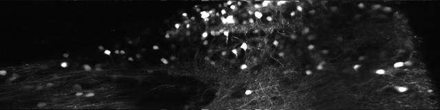
Clearly, the left and right side of the picture are streched out. This does not worry me if I only want to extract fluoresence time courses of neuronal ROIs; but it is a problem for nice-looking pictures that want to have a valid scalebar. Unfortunately, I didn’t find any script in the internet on how un-distorting is normally being done for resonant scanning, so I want to present my own (Matlab) solution for other people looking around. It is not elegant, but it works. For the final solution, scroll to the bottom of the blog entry.

The script uses the input image XX and undistorts the x-direction (2nd dimension of the matrix), yielding the output matrix X. The resulting width in x of the image is adjusted to achieve isotropic resolution in x and y – the conversion factor (xy_conversionfactor) should be around 1 (it is not exactly 1 for my example).

I’m using a ~8 kHz scanner, but the data are sampled only during a fraction of the line time of ca. 63 us, namely the center fraction of of the line time, consisting of 4096 data points, i.e. line dwell time = 4096/80e6 sec < 63 us.

The undistortion follows the inverse of the movement of the resonant scanning. The movement of the scanner is given by a sine/cosine-shape (cos(t*2*pi*f_res) ).

function X = unwarp(XX)

pxperline = size(XX,2); % pixel per line
xy_conversionfactor = 477/512; % empirical xy aspect ratio
pxperline_new = pxperline*xy_conversionfactor;
f_res = 7.91e3; % resonant scanning frequency
linetime = 1/f_res/2;

linedwelltime = linetime*4096/(80e6/f_res/2); % in toto
t_offset = (linetime - linedwelltime)/2;

x = 1:pxperline;
t = t_offset + x/pxperline*linedwelltime;
y  = cos(t*2*pi*f_res);

yy = y - min(y); yy = 1+(yy/max(yy)*(pxperline_new-1));
yy = yy(end:-1:1);
xpos_LUT = interp1(yy,x,1:pxperline_new);
XX_reshaped = reshape(shiftdim(XX,1),size(XX,2),[]);
X = interp1(1:pxperline,XX_reshaped,xpos_LUT,'linear');
X = reshape(X,pxperline_new,size(XX,3),size(XX,1));
X = shiftdim(X,2);
end

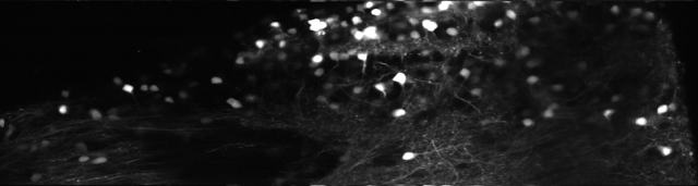
The line starting with “yy =” involves the typical indexing mess that is required to ensure nice behavior at the boundaries of the image. Here is the result:

However, it is worth having a closer look. Can this spatial distortion make data worse? In some sense, yes. If you look at how random noise from a 512×512 image transforms, you see some obvious stripes.When averaging over the columns of the picture, no difference in the mean can be seen. But a look at the column-wise standard deviation reveals that there is something happening when going along the x-axis. This is due to the fact that the signal-to-noise is not the same for all pixel columns of the unwarped image, also due to the interpolation process. Interestingly, this is an effect that can be visible to the eye also for heavily averaged images (especially when using non-linear colormaps as jet, but also for grayscale colormaps), and it is even more visible in single images or movies with lower signal-to-noise.

There’s a way to improve this issue: replacing the interpolation by simply binning the intensity to pixel-bins; e.g. an intensity value of the original image that is mapped to pixel 322.32 in the new image, 68% of the intensity would be assigned to px 322 and 32% to px 323. This is more precise than interpolation and takes better advantage of the available data points. Here is the code:

function X = unwarp_better(XX)

pxperline = size(XX,2); % pixel per line
xy_conversionfactor = 477/512; % empirically found through calibration for my setup
pxperline_new = pxperline*xy_conversionfactor;
f_res = 7.91e3; % resonant scanning frequency
linetime = 1/f_res/2;

linedwelltime = linetime*4096/(80e6/f_res/2); % in toto
t_offset = (linetime - linedwelltime)/2;

x = 1:pxperline;
t = t_offset + x/pxperline*linedwelltime;
y  = cos(t*2*pi*f_res);

yy = y - min(y); yy = 1+(yy/max(yy)*(pxperline_new-1));
yy = yy(end:-1:1);
yy_floor = floor(yy);
yy_remainder = yy - yy_floor; % which fraction goes to the left/right pixel?

X = zeros(size(XX,1),pxperline_new,size(XX,3));
histX = zeros(size(XX,1),pxperline_new);
for k = 1:numel(yy_floor) % split each pixel into the two bins of the new grid
    X(:,yy_floor(k),:) = X(:,yy_floor(k),:) + XX(:,k,:)*(1-yy_remainder(k));
    histX(:,yy_floor(k)) = histX(:,yy_floor(k)) + (1-yy_remainder(k));
    if k < numel(yy_floor)
        X(:,yy_floor(k)+1,:) = X(:,yy_floor(k)+1,:) + XX(:,k+1,:)*yy_remainder(k);
        histX(:,yy_floor(k)+1) = histX(:,yy_floor(k)+1) + yy_remainder(k);
    end
end
X = X./repmat(histX,[1 1 size(X,3)]); % normalize
end

The undistorted brain picture from above looks almost the same because of the good signal-to-noise of the image, but the unwarped noise definitely looks better:As always, it is the details that matter!