As many neuroscientists, I’m also interested in artificial neural networks and am curious about deep learning networks. I want to dedicate some blog posts to this topic, in order to 1) approach deep learning from the stupid neuroscientist’s perspective and 2) to get a feeling of what deep networks can and can not do. Part I, Part II, Part IV, Part IVb. [Also check out this blog post on feature visualization; and I can recommend this review article.]

The main asset of deep convolutional neural networks (CNNs) is their performance; their main disadvantage is that they can be used with profit, but not really understood. Even very basic questions like ‘why do we use rectified linear units (RELUs) as activation functions instead of slightly smoothed versions?’ are not really understood. Additionally, after learning the network is a black box that performs exceedingly well, but one cannot see why. Or, it performs badly, and also to sometimes cryptic reasons. What has the network learned actually?

But there are some approaches that shed light on what has been learnt be CNNs. For example, there is a paper by Matthew Zeiler. I’ve mentioned a Youtube-Video by him in a previous post (link to video). He uses a de-convolution (so to say, a reverse convolution) algorithm to infer the preferred activation pattern of ‘neurons’ somewhere in the network. For neurons of the first layer, he sees very simple patterns (e.g. edges), with the patterns getting more complex for intermediate (e.g. spirals) and higher layers (e.g. dog face). The parallels to the ventral visual stream in higher mammals is quite obvious.

Google DeepDream goes into the same direction, but yielding more fascinating pictures. Basically, the researchers took single ‘neurons’ (or a set of neurons encoding e.g. animals) in the network and used a search algorithm to find images that activate this ‘neuron’ most. The search algorithm can use random noise as a starting point, or an image provided by the user. Finally, this leads to the beautiful pictures that are well-known by now (link to some beautiful images). Google has also released the source code, but within the framework of Caffè (link), and not Tensorflow. However, at the bottom line of this website, they promise to provide a version for Tensorflow soon as well [Update October 2016: It has been released now].

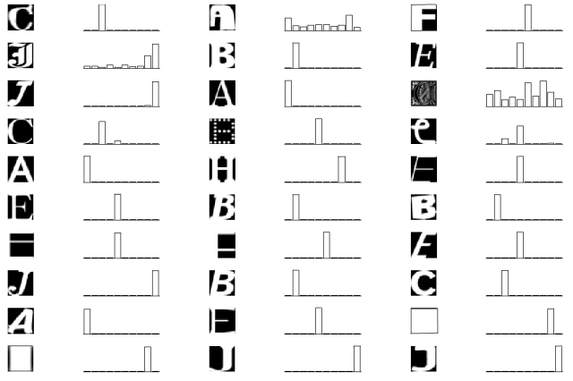
In the meantime, let’s have a less elaborate, but more naïve look, in order to get a better understanding of deep networks. I will try to dissect parts of a 5-layer convolutional network that I wrote during the Tensorflow Udacity course mentioned previously in this blog. For training, it uses a MNIST-like data, but a little bit more difficult. The task is to assign a 28×28 px image to one of the letters A-J. Here you can see how the network performs for some random test data. In the bar plot, the positions 1-10 correspond to the letters A-J, visualizing the certainty of the network.

So let’s look inside the black box. The first layer in this network consists of sixteen 5×5 convolutional filters. Those filters had been established during learning. Here they are:

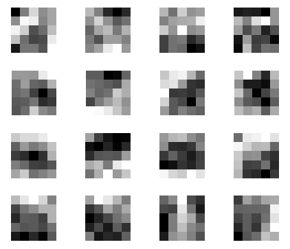
Does this make sense to you? If not, here are the 16 filters (repeatedly) applied to noise, revealing the structures that are made to detect:

Obviously, most of those filters have a preference for some (curved) edge elements (which is not really surprising).

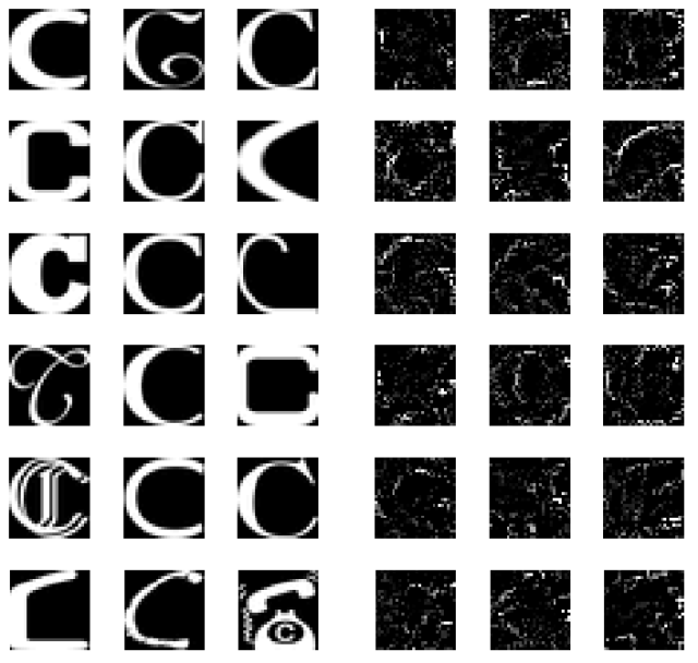
For simple networks like this one, which is not very deep and only has to learn simple letters, intermediate layers do not really represent something fancy (like spirals, stars or eyes). But one can at least have a look at how the ‘representation’ of the fifth layer, the output layer looks like. For example, what is the preferred input pattern of the output ‘neuron’ that has learned to assign the letter ‘C’?

To find this out, I used the same deep learning network as before, but kept constant the network weights that had been learnt before. Instead, I varied the input image, whilst telling the stochastic gradient descent optimizer to maximize the output of the ‘C’ neuron.

Starting from random noise, different local optimization maxima are reached, each of them corresponding more or less to an ‘idea of C’ that the deep network has in mind. The left side shows ‘C’s from the original dataset. The right hand side shows ideas of ‘C’ that I extracted from the network with my (crude) search algorithm. One obvious observation is that the extracted ‘C’s do not care about surfaces, but rather about edges, which can be expected from a convolutional network and from the filters of the first layer shown above.