Interesting papers on behavioral timescale synaptic plasticity (experiments)

Behavioral timescale synaptic plasticity (BTSP) is a form of single-shot learning observed in hippocampal place cells in mice (Bittner et al., 2015, 2017). The idea is that post-synaptic activations (“eligibility traces”) are potentiated by a dendritic plateau potential/burst (“instructive signal”) that comes up to several seconds after the first signal. This result turned out to be one of the most reproducible findings of recent systems neuroscience, being replicable across labs and across stimulation protocols (via single-cell electrophysiology (Bittner et al., 2015) but also via optogenetic induction (O’Hare et al., 2022)). Many different labs are working in this interesting field, and here are a few recent papers on this topic.

A role for CaMKII in BTSP

Xiao et al. (2023) from the Magee lab report on a “critical role for CaMKII” in BTSP. “CaMKII” is known as a promotor fragment that is specific for excitatory neurons, but CaMKII is more than that – CaMKII is a calcium-dependent kinase (but see the recent paper by Tullis et al. (2023)) with important functions for plasticity. After phosphorylation, CaMKII remains in this activated state for several seconds and is therefore a candidate actor for BTSP, which acts on a timescale of several seconds as well. I learnt from this paper’s introduction that there is a CaMKII sensor based on FRET which revealed a shorter decay time for CaMKII’s phosphorylated state when it carried a specific mutation in CaMKII.

The authors take advantage of an established mouse line with this specific mutation, which resulted in deficits of memory and synaptic plasticity. Xiao et al. found, using in vivo patch clamp, that BTSP was prevented or reduced in these mutated mice (Fig. 3), suggesting an indeed critical role of CaMKII for the induction of BTSP.

As a side-finding, the authors describe that intrinsic burst propensities of CA1 neurons were quite different for mutants and wildtypes (unfortunately, they only show few example traces of such bursts), and they follow up on this result by characterizing the intrinsic properties in slices.
A question that came up and was partially addressed by the authors are the possible side-effects of chronically mutated CaMKII on the entire development and on other brain regions or also the hippocampus before the start of the experiment. However, the main finding of the manuscript (prevention of BTSP in CaMKII-mutated mice) seems to be solid despite these non-avoidable confounds. Of course, the study does not address how exactly CaMKII is involved in BTSP. The way to address this question will probably require using fluorescent reporters of CaMKII activity and very tedious dissection of molecular signaling pathways.

Monitoring of place cell induction via BTSP with calcium imaging

Grienberger and Magee (2022) conducted a simple and elegant study using calcium imaging that confirms and connects previous ideas on hippocampal plasticity and BTSP.
It had been known since a long time that hippocampal place cells are more abundant around more important locations, for example, reward locations. Here, the authors observe the transition from similar representation of all locations towards preferred representation of reward location using calcium imaging. They find evidence that this transition is induced by BTSP. To this end, they identify putative BTSP burst events in single neurons from calcium imaging data and track the activities of these neurons before and after such burst events. Moreover, they use optogenetics to show that input from entorhinal cortex (EC3) is required for the transformation of equal to reward-preferring representation of space. This finding is in line with the existing ideas about EC3 projections to provide the instructive signal that triggers bursts in apical dendrites and BTSP in CA1 neurons.

One of the most critical parts of this study is the identification of bursts to induce place fields using calcium imaging (in previous studies, this was usually done by in vivo whole-cell recordings). There is some uncertainty about the identification of these induction events (see the “CA1 place cell identification” subsection in the Methods section; check out a more recent preprint by the same lab, which uses much more complex criteria to detect BTSP events from calcium imaging; see the Methods subsection “BTSP Analysis” from  Vaidya et al. (2023)). It would be very interesting to thoroughly study – for example with simultaneous calcium imaging and single-cell electrophysiology in vivo -, which calcium events correspond to BTSP/burst events and which calcium events correspond to “regular” spiking. However, this seems technically too challenging, and the more ad-hoc methods to identify such events in this study seem fully adequate for the question addressed. P.S. If you find this paper interesting, check out the publicly available reviewer reports.

Voltage imaging of BTSP with optogenetic perturbations

Fan et al. (2023) use an impressive combination of voltage imaging and optogenetics techniques in vivo to study BTSP. Let me cite the abstract to give an idea about the methodological craziness of this study: “We combined genetically targeted voltage imaging with targeted optogenetic activation and silencing of pre- and post-synaptic neurons to study the mechanisms underlying hippocampal behavioral timescale plasticity.” Optogenetic induction of place cells in hippocampus has been done before, but not combined with voltage imaging. This together with simultaneous silencing of specific projections sounds like a completely crazy project. Several interesting findings: Excitability of pyramidal neurons (as measured with combined optogenetic activation and voltage imaging) did not increase upon BTSP. CA2/3 to CA1 inputs were potentiated upon BTSP (optogenetic activation of, although only contralateral, CA2/3 with a fiber during voltage imaging of CA1 neurons). And the activity of CA2/3 cells projecting to CA1 was required for BTSP (optogenetic silencing of projection-specific CA2/3 neurons while voltage imaging in CA1).

Overall, I would have loved to read more about these experiments and their interpretation.
Grienberger and Magee (2022) showed that (ipsilateral) EC3 input is necessary for BTSP, while Fan et al. (2023) showed that (contralateral) CA2/3 input is required. The idea is that both CA2/3 (for the eligibility trace) and EC3 input (for the instructive signal) are required, and both results are consistent with the standard theory of BTSP. It is only a bit surprising that even the contralateral CA2/3 input, as reported by Fan et al. was sufficient. In their study, the contralateral side was inhibited to enable fiber placement at CA2/3 and voltage imaging in CA1. This must be kept in mind because the authors, to access CA1 with 1P voltage imaging, also removed the central part of the external capsule; I wonder whether this removed part of the corpus callosum does not contain some of these contralateral projections.

A plasticity rule in cortex reminiscent of BTSP

Caya-Bissonnette et al. (2023) from Jean-Claude Béïque’s lab in Ottawa used slice physiology and modeling to show that a variant of BTSP exists in layer 5 pyramidal cells of cortex (S1) in mice. I have to admit that the often very long and complicated sentences in the Results section and the slightly overcrowded figures make it a tough paper to read, but it is worth it.

The authors use pre- and post-synaptic stimulation pairing paradigms as they were used extensively since the 1990s – but with the crucial difference that pre- and post-synaptic events were not separated by milliseconds but by 0.5-1.0 s. Using this approach, they found a potentiation of synapses that did not depend on the temporal order of pre/post stimulation. Therefore, they call this plasticity rule “associative”. The authors furthermore show that the endoplasmic reticulum (ER, reminiscent of O’Hare et al. (2022)) and several related calcium signaling pathways are involved in the latent “eligibility trace” that holds the memory of first stimulation before the second stimulation arrives, by extending the decay time constant of calcium (Fig. 4). The decay time is not extended by much, but maybe this slight increase is enough to induce plasticity.

Altogether, this is a very interesting study focusing on slice physiology. On one side, this is a limitation since the paper claims to have found a cortical variant of hippocampal BTSP, an effect that was primarily convincing because it had been shown in behaving animals. Therefore, one should critically inspect the choices of the plasticity protocol. For example, I noticed that the authors used a 10×20 Hz stimulation that seemed to me maybe a bit too strong and repetitive a stimulation and does not resemble typical BTSP events in vivo; moreover, during BTSP events, bursting and the associated plateau potentials were shown to be involved in the post-synaptic not the pre-synaptic cell in vivo (Bittner et al., 2015). Maybe I missed it, but I did not find this aspect discussed in the paper.

On the other side, the study is, despite this limitation, very interesting since it demonstrates how powerful slice physiology can be and how much we miss by only focusing on processes accessible in vivo. Moreover, it shows under which condition a classical STDP protocol can be transformed into a longer-timescale “BTSP” (Fig. 1F). To my knowledge, a plasticity rule with such long delays has not been convincingly demonstrated in cortex before, neither in slices nor in vivo. It may be a stretch to call the observed effect “BTSP”, drawing the analogy to the results seen in hippocampus in vivo, thereby gradually diluting the meaning of “BTSP”. However, this is just naming conventions – the science in the paper is interesting.

That’s it from my side about interesting papers on behavioral timescale synaptic plasticity.

Did I miss an interesting recent paper on this topic? Let me know in the comments!

References:

Bittner, K.C., Grienberger, C., Vaidya, S.P., Milstein, A.D., Macklin, J.J., Suh, J., Tonegawa, S., Magee, J.C., 2015. Conjunctive input processing drives feature selectivity in hippocampal CA1 neurons. Nat. Neurosci. 18, 1133–1142. https://doi.org/10.1038/nn.4062

Bittner, K.C., Milstein, A.D., Grienberger, C., Romani, S., Magee, J.C., 2017. Behavioral time scale synaptic plasticity underlies CA1 place fields. Science 357, 1033–1036. https://doi.org/10.1126/science.aan3846

Caya-Bissonnette, L., Naud, R., Béïque, J.-C., 2023. Cellular Substrate of Eligibility Traces. https://doi.org/10.1101/2023.06.29.547097

Fan, L.Z., Kim, D.K., Jennings, J.H., Tian, H., Wang, P.Y., Ramakrishnan, C., Randles, S., Sun, Y., Thadhani, E., Kim, Y.S., Quirin, S., Giocomo, L., Cohen, A.E., Deisseroth, K., 2023. All-optical physiology resolves a synaptic basis for behavioral timescale plasticity. Cell 186, 543-559.e19. https://doi.org/10.1016/j.cell.2022.12.035

Grienberger, C., Magee, J.C., 2022. Entorhinal cortex directs learning-related changes in CA1 representations. Nature 611, 554–562. https://doi.org/10.1038/s41586-022-05378-6

O’Hare, J.K., Gonzalez, K.C., Herrlinger, S.A., Hirabayashi, Y., Hewitt, V.L., Blockus, H., Szoboszlay, M., Rolotti, S.V., Geiller, T.C., Negrean, A., Chelur, V., Polleux, F., Losonczy, A., 2022. Compartment-specific tuning of dendritic feature selectivity by intracellular Ca2+ release. Science 375, eabm1670. https://doi.org/10.1126/science.abm1670

Tullis, J.E., Larsen, M.E., Rumian, N.L., Freund, R.K., Boxer, E.E., Brown, C.N., Coultrap, S.J., Schulman, H., Aoto, J., Dell’Acqua, M.L., Bayer, K.U., 2023. LTP induction by structural rather than enzymatic functions of CaMKII. Nature 621, 1–8. https://doi.org/10.1038/s41586-023-06465-y

Vaidya, S.P., Chitwood, R.A., Magee, J.C., 2023. The formation of an expanding memory representation in the hippocampus. https://doi.org/10.1101/2023.02.01.526663

Xiao, K., Li, Y., Chitwood, R.A., Magee, J.C., 2023. A critical role for CaMKII in behavioral timescale synaptic plasticity in hippocampal CA1 pyramidal neurons. https://doi.org/10.1101/2023.04.18.537377

Posted in Calcium Imaging, Data analysis, electrophysiology, Network analysis, Neuronal activity, Reviews | Tagged , , , | 4 Comments

Interesting papers on recent neuroscience methods

Find below three interesting methods papers relevant for neuroscience. All three of them are, in my opinion, worth a quick read.

Acoustic cameras to localize ultrasound vocalization of mice

Sterling et al. (2023) from the lab of Bernhard Englitz addressed the problem how to localize ultrasound vocalizations (USVs) from rodents, in particular mice. The localization of USVs and their reliable attribution to a specific mouse can be challenging, especially when mice are interacting snout-to-snout. The authors managed to perform sound localization with a precision of less than 5 mm (91% of USVs correctly assigned). How do they achieve this?

The authors combined two complementary approaches. In a first approach, they used an “acoustic camera” formed by an 8×8 array of 64 ultrasound microphones (https://sorama.eu/products/cam64). This approach provided spatially precise localization but was less reliable for high frequencies. In a second approach, they used an array of only 4 but high-quality ultrasound microphones (https://www.avisoft.com/). Figure supplement 1-1 nicely compares the noise spectra of these two microphone types. The second approach was more important to detect USV events, while the “acoustic camera” approach was essential for localization of the detected events. A nice methods paper!

Glyoxal fixation for improved antibody staining

In this study, Konno et al. (2023) from the lab of Masahiko Watanabe refined and tested an alternative protocol for immunohistochemistry (IHC), following up on a study by Richter et al. (2018). The authors replaced the standard fixative (4% paraformaldehyde, PFA) by a different solution (glyoxal) and find that this modified fixation protocol enables improved diffusion of and labeling with antibodies, including antibodies against important proteins such as synaptic adhesion molecules, receptor proteins and ion channels.

The authors mention a few caveats in the Discussion: Glyoxal fixation improved signal for certain antibodies but not for all, without an indication why this could be the case. The sample seemed to be less than hard and fixed for glyoxal than for PFA fixation. Moreover, they report that “ultrastructural images of neurons and synapses” were more strongly compromised by glyoxal fixation compared to PFA fixation. This last comment seems interesting, since Richter et al. (2018) in their original publication on glyoxal fixation stated that ultrastructure was better conserved in glyoxal than in PFA. I’m curious whether glyoxal might become the new standard for IHC during the next decade!

Near-infrared co-illumination protects fluorophores

Fluorescence occurs when fluorophore molecules transition into an excited state and, during the relaxation process into the ground state, release a photon. This process can go awry when the molecule transitions from the excited state into a dark (triplet) state or other non-desired states where the molecule is stuck (photobleaching) or which result in chemical reactions that generate oxidative stress (phototoxicity). As an experimentalist, it is essential to find the balance between (a) as much power as necessary (to be able to observe the structures of interest) and (b) as little power as possible (to prevent bleaching and toxicity).

In a surprising study, Ludvikova et al. (2023) find that near-infrared (NIR) light prevents photobleaching and phototoxicity. The authors performed imaging of standard fluorescent proteins (EGFP) in cell culture using one-photon widefield microscopy with an excitation wavelength of around 470 nm. They find that co-illumination with NIR light (approx. 900 nm) reduced bleaching induced by 470 nm. It is not fully clear from the study why NIR co-illumination prevents transitioning into triplet states, but the evidence that this indeed happens seems very convincing.

It would be interesting to see how this can be generalized to different illumination intensities and patterns, e.g., to confocal or light-sheet microscopy. And it poses the intriguing question whether two-photon microscopy of green fluorophores, which typically uses a wavelength in the NIR (around 920 nm), also takes advantage of this protective effect. For two-photon microscopy, illumination already occurs at around 900 nm, so it could be that the same photons that induce fluorescence also protect from bleaching/toxicity. It seems however challenging to test this hypothesis experimentally. As a sidenote, I’m reminded of my own experiments (reported in this blog post) where I found that long-lived dark triplet states seemed to be less relevant at 920 nm than predicted from experiments performed at 800 nm. I’m hoping that follow-up studies will further dissect the NIR co-illumination effect and study its relevance for other imaging modalities, especially confocal and light-sheet imaging!

References

Konno, K., Yamasaki, M., Miyazaki, T., Watanabe, M., 2023. Glyoxal fixation: An approach to solve immunohistochemical problem in neuroscience research. Sci. Adv. 9, eadf7084. https://doi.org/10.1126/sciadv.adf7084

Ludvikova, L., Simon, E., Deygas, M., Panier, T., Plamont, M.-A., Ollion, J., Tebo, A., Piel, M., Jullien, L., Robert, L., Le Saux, T., Espagne, A., 2023. Near-infrared co-illumination of fluorescent proteins reduces photobleaching and phototoxicity. Nat. Biotechnol. 1–5. https://doi.org/10.1038/s41587-023-01893-7

Richter, K.N., Revelo, N.H., Seitz, K.J., Helm, M.S., Sarkar, D., Saleeb, R.S., D’Este, E., Eberle, J., Wagner, E., Vogl, C., Lazaro, D.F., Richter, F., Coy-Vergara, J., Coceano, G., Boyden, E.S., Duncan, R.R., Hell, S.W., Lauterbach, M.A., Lehnart, S.E., Moser, T., Outeiro, T.F., Rehling, P., Schwappach, B., Testa, I., Zapiec, B., Rizzoli, S.O., 2018. Glyoxal as an alternative fixative to formaldehyde in immunostaining and super-resolution microscopy. EMBO J. 37, 139–159. https://doi.org/10.15252/embj.201695709

Sterling, M.L., Teunisse, R., Englitz, B., 2023. Rodent ultrasonic vocal interaction resolved with millimeter precision using hybrid beamforming. eLife 12, e86126. https://doi.org/10.7554/eLife.86126

Posted in Data analysis, Imaging, Microscopy, neuroscience, Reviews | Tagged , , | Leave a comment

Interesting papers on online motion correction for calcium imaging

In a living animal, the brain is moving up and down in the skull. This brain motion can be due to breathing, heartbeat, tongue movements, but also due to changes of posture or running. For each brain region and posture, specific brain movements are more likely to occur. For imaging of neuronal activity using two-photon microscopy through a window, the coverslip glass is usually gently pressed onto the brain to reduce motion. As a consequence, brain motion is typically smaller close to the glass surface and becomes more prominent for imaging deeper below the surface.

Why axial movement artifacts are bad

From the point of view of data analysis, there are two fundamentally different types of brain movements: Lateral movements (within the xy-imaging plane) and axial movement (in the axial z-direction). The first type can be corrected (except in the boundary region of the FOV) by shifting the image back to the “right place” within the plane. Axial movement, on the other hand, shifts the imaging focus to a different depth and cannot be corrected. From my experience, these axial motion artifacts are often underestimated and often ignored. But even if they are small (and barely visible by eye after non-rigid xy-motion correction), they might have an effect when an analysis averages across a lot of repetitions or “trials”. Especially for low imaging resolution and low signal-to-noise, it is often difficult to judge by eye whether something was due to z-motion or due to neuronal activity related to movement (or due to both). Imaging of small structures like axons or laterally-spreading dendrites is especially prone to movement artifacts, and there are many additional edge cases where brain movement might influence the analysis. Ideally, one would be able to correct for z-motion online during the recording. For example, when the brain moves up by 5 µm, the focus of the microscope would move up by the same amount, therefore imaging the same tissue despite the motion. Typically, z-motion of the brain is relatively slow, often below 20 Hz in mice. An online motion correction algorithm would therefore be required to work at a temporal responsiveness of, let’s say 40-50 Hz.

ECG-synchronized image acquisition

There have been several suggested methods to solve this problem. Paukert and Bergles (2012) developed a method to correct for only lateral (and not axial) movement, but the methods is still worth mentioning. They recorded the electro-cardiogram (ECG) and used the peak of the R-wave to reliable trigger image acquisition. Therefore, they did not really correct for heartbeat-induced motion but rather recorded such that brain motion was the same for all acquired imaging frames. Better imaging preparations (more pressure exerted onto the brain by the coverslip window) have made this approach less relevant for cortical imaging. However, for deeper imaging, e.g., with 3P microscopy, the stabilization through the coverslip is reduced. Therefore, Streich et al. (2021) used ECG-synchronized 3P scanning to improve image quality. They went a few steps further than Paukert and Bergles (2012) using the past heartbeats to predict – online with an FPGA – the next R-wave and to stop image acquisition around the R-wave window.

Correction of stereotypic axial motion with an ETL

A conceptually similar method has been developed by Chen et al. (2013). They also wanted to avoid motion artifacts induced by clearly defined motion-related events – not heartbeats in this case, but licking events. Depending on the brain region and the effort the mouse has to make, licking can cause huge motion artifacts. Chen et al. (2013) did not want to stop imaging during licking but instead wanted to correct the axial focus using a electrically tunable lens (ETL). They observed that licks consistently changed the focus of the imaging plane. They therefore used a lick sensor and fed its output to a corrective signal that moved the focus of the ETL in a calibrated manner. The idea is therefore based on the assumption that lick-induced movement is stereotyped. Therefore, one might have to recalibrate the correction algorithm for each mouse or for motion due to other parts of the body. However, it is, to my knowledge, the first attempt to really correct for axial brain motion in vivo.
It would be interesting to combine the recording of more diverse behaviors using a video camera with fast processing and with a predictive component as by Streich et al. (2021) to develop a more general brain movement predictor and corrector. For example, an algorithm could map behaviors to expected brain movements for 10 min and then perform recordings with perfectly predicted brain motion that can be anticipated and corrected by an ETL or another remote scanning device. Wouldn’t this be cool?

Using the sample surface as a reference

Another set of methods tries to image the brain and at the same time perform a scan of a reference object in the brain (a “guide star”), or the brain surface or the brain itself, in order to extract the desired corrective factor for scanning in real-time.
Laffray et al. (2011) used a reflective imaging modality to detect the position of the spinal cord (which is well known to move a lot!). In their approach, they only corrected for lateral brain motion, most likely because their microscope was not equipped with a z-scanning device. But it seems possible to generalize this method to axial movement correction as well. The limitation of this approach is that the brain surface is typically pressured by a coverslip and does not move so much – it is rather the deeper parts of the brain that move much more.

Scanning a reference object with an AOD scope

A technically more advanced method for real-time 3D movement correction was developed by Griffiths et al. (2020). In this study, the authors used a random-access AOD-based microscope, recording only small environments around single neurons. Therefore, post-hoc movement correction, also in the lateral direction, was not really an option. To address this problem, the authors developed a closed-loop system based on an FPGA to perform online motion correction. AODs (acousto-optic deflectors) are very fast scanners, so the scan speed is not an issue. The authors defined a 3D reference object that was scanned in parallel to the imaged neurons, and corrected the focus of the microscope according to movements of the reference object. This method seems to be very elegant. The only limitation that I can see is that it requires an AOD microscope – very few z-scanning techniques would be able to perform an ultra-fast z-scan as a reference (maybe TAG-lenses would be an option?). And AOD scopes have been long known to be very challenging to operate and align – although some companies seem to have managed to make the systems a bit more user-friendly during the last decade.

Scanning the brain with OCT-based imaging

Recently, I came across another paper about online movement correction, by Tucker et al., (2023). The authors used optical coherence tomography to measure brain motion and to online correct for it. In this paper, the authors present a method to correct for brain motion in x and y, not addressing the more relevant problem of z-motion (although this is discussed in depth as well). On a side-note, I noticed that corrections were applied by adding signals to the regular voltage signals used to drive the scan mirrors, reminding me of my simple solution a few years ago to add two analog signals with a summing amplifier. Anyway, a z-correction would be more difficult to implement in a standard microscope because it would require an existing z-scanning device (such as a remote z-scanner, a tunable lens, or a piezo attached to the objective). However, I found the idea compelling, and on paper the principle of OCT seems simple. An OCT is more or less an interferometer that uses infrared backscattered light to form an image. Imaging speed is high for the modern variants of OCT imaging, and the possible resolution seems to be around 1 μm. If you now have become interested in OCT, I can recommend this introduction, especially section 2.3 on “Signal formation in OCT”.

Open questions about OCT for online motion correction

Unfortunately, I have never seen or used an OCT microscope before. Therefore, I have no intuition how difficult it would be to achieve high-resolution OCT imaging. How does an OCT volumetric image of a mouse brain look like? Which structures in the brain generate the contrast? Is there any contrast? How long does it take to acquire such an image with sufficient contrast at high resolution? What is the price tag of a spectral-domain OCT system? Is it more or less difficult to build than e.g. a two-photon microscope?
I have the impression that the study by Tucker et al. (2023) only scratches the surface of what is possible, and that OCT imaging could be combined with 2P imaging without compromising excitation or detection pathways. If you are an expert in this technique and happen to meet me at the next conference, I’d be interested in knowing more!

P.S. Did I miss an interesting paper on this topic? Let me know!

[Update 2023-09-10: Also check out the comment below by Lior Golgher, who brings up additional interesting papers, including approaches to perform volumetric imaging in 3D, which enables post-hoc motion correction in the axial direction or the selction of a more motion-robust selection of an extended 3D-ROI.]

References

Chen, J.L., Pfäffli, O.A., Voigt, F.F., Margolis, D.J., Helmchen, F., 2013. Online correction of licking-induced brain motion during two-photon imaging with a tunable lens. J. Physiol. 591, 4689–4698. https://doi.org/10.1113/jphysiol.2013.259804

Griffiths, V.A., Valera, A.M., Lau, J.Y., Roš, H., Younts, T.J., Marin, B., Baragli, C., Coyle, D., Evans, G.J., Konstantinou, G., Koimtzis, T., Nadella, K.M.N.S., Punde, S.A., Kirkby, P.A., Bianco, I.H., Silver, R.A., 2020. Real-time 3D movement correction for two-photon imaging in behaving animals. Nat. Methods 1–8. https://doi.org/10.1038/s41592-020-0851-7

Laffray, S., Pagès, S., Dufour, H., Koninck, P.D., Koninck, Y.D., Côté, D., 2011. Adaptive Movement Compensation for In Vivo Imaging of Fast Cellular Dynamics within a Moving Tissue. PLOS ONE 6, e19928. https://doi.org/10.1371/journal.pone.0019928

Paukert, M., Bergles, D.E., 2012. Reduction of motion artifacts during in vivo two-photon imaging of brain through heartbeat triggered scanning. J. Physiol. 590, 2955–2963. https://doi.org/10.1113/jphysiol.2012.228114

Streich, L., Boffi, J.C., Wang, L., Alhalaseh, K., Barbieri, M., Rehm, R., Deivasigamani, S., Gross, C.T., Agarwal, A., Prevedel, R., 2021. High-resolution structural and functional deep brain imaging using adaptive optics three-photon microscopy. Nat. Methods 18, 1253–1258. https://doi.org/10.1038/s41592-021-01257-6

Tucker, S.S., Giblin, J.T., Kiliç, K., Chen, A., Tang, J., Boas, D.A., 2023. Optical coherence tomography-based design for a real-time motion corrected scanning microscope. Opt. Lett. 48, 3805–3808. https://doi.org/10.1364/OL.490087

Posted in Calcium Imaging, Data analysis, Imaging, machine learning, Microscopy, Neuronal activity, neuroscience | Tagged , , , , | 4 Comments

The idea for a journal “eLife-A”

The process of publishing and reviewing scientific results is often a strange and difficult-to-navigate landscape.

It would take too long to mention all the problems and pitfalls related to publishing. For example: overly high publication charges; long turnaround times for reviews and editorial decisions; incomprehensible reviews; incomprehensible manuscripts; delayed careers due to rejections and revision processes; lack of transparency of manuscript evaluation; lack of open access. Just to name what comes to my mind immediately.

Some of these issues have been partly addressed during the last decade by preprints (arXiv and bioRxiv), open reviews (check out my previous blog post on public peer reviews), non-legal mirrors of closed-source material (sci-hub) and experiments with new publication models (most prominently, the new eLife publication model).

Since the inception of eLife’s new publication model End of 2022, the first papers have now gone through this process, and I have the overall impression that the model is mostly well-received and definitely worth the experiment. The published papers now not only include the public peer reviews, but also an assessment by the editors, which summarizes and evaluates the claims of the paper. Manuel Schottdorf just pointed out to me that this digest can also be an outright negative assessment, for example concluding that “the evidence” for the claims is “considered inadequate” (full article plus assessment)! That’s impressive! Even though such an assessment might appear harsh from the authors’ side, such an open process makes science itself and its progress more transparent. The specific paper is outside my area of expertise, but I like the idea in general. The conclusions and claims of a paper should not be evaluated based on its association with a specific journal, but based on its assessments by expert reviewers.

In a post on Twitter, Aaron Milstein just put forward a suggestion to implement this assessment in a way that is also readable by evaluation and grant committees: by giving to each paper a grade between “A” and “F”.

For example, “eLife-A” would correspond to “Nature/Science/Cell” in terms of broad relevance, “eLife-B” to “Nature Neuroscience” or “Neuron”, “eLife-C” maybe to the current version of eLife, and so on.

Personally, I do not like the US grading scheme (from A to F), and I’m also a bit skeptical about mixing impact/relevance and methodological rigor/correctness – I really hate high-impact papers with strong claims that are not supported or only weakly supported by data, but I know that many people think differently. In any way, a one-dimensional metric (from A to F) would certainly benefit from improved interpretability, which is already better than what we have right now.

I could also imagine that as a further step, a retrospective re-evaluation of specific papers could be possible, with this secondary, retrospective evaluation reflecting the impact a paper had on its field. It is easier to tag an existing paper that already has a specific “rating” with a new additional “post-publication review rating”, rather than saying that “in retrospect, this Scientific Reports paper should have been published in Nature”. But this is just a side-note.

In an ideal scenario, such a publication model would be set up by an independent entity. eLife would actually be a good choice, because its publication model is already very close to this model. Alternatively, the EU funding agencies or the NIH could set up such a journal and oblige all projects funded by EU or NIH to publish in this journal.

One of the several positive and less obvious side-effects would be to prevent journal hopping. Journal hopping is the process of sequentially submitting a paper to several high-impact journals, in the hope of being lucky with one of them. This process not only wastes a lot of resources from both journals and voluntary reviewers but also comes at the cost of junior researchers whose careers are delayed to an unnecessary degree by this process.

I really hope that a publication scheme that gets rid of the journal tags and replaces them with grades (=subjournals) becomes a reality soon. I think it is a good idea.

Posted in Reviews | Tagged , | 2 Comments

Annual report of my intuition about the brain (2022)

How does the brain work and how can we understand it? To view this big question from a broad perspective at the end of each year, I’m reporting some of the thoughts about the brain that marked me most during the past twelve month – with the hope to advance and structure the progress in the part of my understanding of the brain that is not immediately reflected in journal publications. Enjoy the read! And check out previous year-end write-ups: 2018201920202021, 2022, 2023, 2024.

During the last years’ write-ups, I have been thinking about experiments to study self-organized plasticity in living brains. This year, I have been busy with preparations for the implementation of this line of research and hope to be working on it next year. Experimentally, I have been mostly occupied with – and more and more intrigued by – the study of hippocampal astrocytes and how they integrate calcium signals. In experiments connected to this project, we are now studying the role of neuromodulation and the locus coeruleus in more detail. And I’m glad that I can learn more about this interesting brain area by doing experiments myself. But I will discuss this in another blog post in more detail.

For this write-up, I want to discuss a small subfield of neuroscience that I only became aware of this autumn and that is closely related to ideas of self-organized neuronal networks: the experimental study of learning in cell cultures. How can the neuronal system of a cell culture be used to interact with a (virtual) world in a closed loop? In this blog post, I will discuss a few important papers to understand what can be studied with this model system of learning.

In conclusion, I think that this field is interesting in principle, as it provides a method to study plasticity (although this is not necessarily the primary aim of this kind of research). The method suffers from the problem, as most in vitro slice approaches as well, that experimental protocols for plasticity induction might be artificial and not related to processes in vivo.

I became aware if the field in October, when a high-profile paper on this topic came out and was prominently covered on social media – partly for making misleading claims and not citing prior research. I want to make it better and start chronologically with a seminal paper from 2001.

A network of cultured cortical neurons is trained to stop a stimulus

Shahaf and Marom showed in 2001 what can be described as “learning-in-a-dish” [1,2]. In these experiments, they grew a culture of cortical neurons on a 2D multi-electrode array (MEA) such that they could both stimulate these neurons and record from them. They used this system to provide some neurons with a specific stimulus. When the neuronal network exhibited a certain firing pattern briefly after stimulation, the stimulation was stopped. With this approach, the cultured network was embedded in a closed-cloop interaction.

Interestingly, the cultured network indeed started to increasingly show these spiking patterns that stopped the external stimulation. The observation is very easily summarized by figure 2 in their experimental paper [1]. After learning, the network is much more activate in a pre-defined time window (shaded area), thereby shutting down the stimulation:

This is a fascinating and also surprising observation. It seems as if the network is realizing that there is a stimulus, decides that the stimulus is annoying and therefore puts forward measures to stop and prevent the stimulus. Such a description is however highly anthropomorphic and does not really help to understand what is going on.

According to Shahaf and Marom, their observation shows in the first place that a neuronal network does not depend on a distinct implementation of reward or other forms of reinforcement. Instead, the network, following Shahaf and Marom, explores configurations until a desired state is reached (in this case: the state of stimulus removal) [1]. The authors discuss the implications a bit more in detail in [2] (check out section 7) but remain rather vague on the possible mechanisms of synaptic plasticity that might underlie such behavior.

A network of cultured cortical neurons interacts with a virtual world

Going slightly beyond the very simple closed loop by Shahaf and Marom, researchers from the lab of Steve Potter, which according to the lab’s website has “created the field of embodied cultured networks”, used the activity of the cultured neurons to drive the behavior of an “animal” in a virtual world [3]. The sensory feedback received by this animal in the virtual world is fed back to the cultured neurons. In this study, the focus is primarily on showing that it is possible to have a cultured network and a very simple virtual environment in a closed loop. This sounds particularly fascinating as the paper was published during a time when the movie Matrix had just come out.

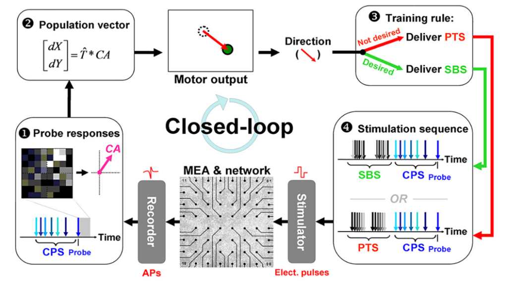
Afterwards, in order to be able to evaluate learning and plasticity systematically, the lab moved to specific tasks based on this experimental design [4]. This study by Bakkum, Chao and Potter is conceptually close to the studies by Shahaf and Marom discussed above. The experimental design is depicted in this nice schematic (part of figure 1 in [4]) and shows a clearly identified mapping of the population activity onto a “motor output”.

Here, SBS (unpatterned shuffled background stimulation) serves as a kind of reward or neutral stimulus while PTS (patterned training stimulation) serves as an aversive stimulus that makes the network provide different output activity patterns. The (unchanging) context-control probing sequence (CPS) is used as a probe, and the network response upon the CPS pattern is regarded as the system’s motor output. Therefore, PTS or SBS act as plasticity- or feedback-stimuli, whereas CPS defines a probing time window to elicit the “motor output”.

The authors show that the networks could learn to provide mostly correct motor output when trained with such a paradigm. In addition, they quantify plasticity processes over time. Plasticity was higher during the learning procedure compared to baseline and remained higher for >1h after training. To summarize, the authors do not dig into mechanisms of cell-to-cell plasticity but rather provide a broader, systemic description of what is going on.

A difficult-to-grasp feature of this experimental study is the design of the patterned training stimulations (PTSs). The authors repeatedly applied different stimulation patterns (e.g., PTS1 stimulates electrodes 1, 4, 7 and 15, PTS2 stimulates electrodes 6, 8, 19, 20, 21 with specific stimulation intensities). Their algorithm was designed to choose from a pool of PTSs and select the PTS that resulted in plasticity towards a network state that generated the desired “motor” output. In 2022, most people (or at least myself) are so much used to deep learning and gradient descent that it is almost strange to read about such a random exploration approach.

Interestingly, the authors also investigated a comparable paradigm in a separate and purely theoretical study [5]. In this study, they replaced the cultured network with a simulated network and found very similar learning compared to the in vitro study. They found that this behavior depended on spike-time dependent plasticity, a cell-to-cell synaptic plasticity rule, and on STD, a short-term plasticity rule that helps to prevent large system-wide bursts.

From my perspective, it is interesting to see that the cell culture results could be replicated with a network that was based on STDP. A large part of the paper however instead focuses on the question how to choose and adapt stimuli that make the network learn the desired output. I would have been interested to get to know more about how STDP is shaped by the stimulation patterns and driven towards the desired output.

Learning by stimulation avoidance and autopoiesis

The group of Takashi Ikegami tried to better understand what is actually going on when neuronal cultures as in the experiments by Shahaf and Marom [1] learn to shut down an external stimulus. They study this effect using simulated neuronal networks and, as in work from the Potter lab [5], they identify spike-timing dependent plasticity (STDP) as an essential factor to mediate this learning process. As in work from the Potter lab, they also use an “embodied” application with a moving simulated robot that learns to avoid walls [6].

The main take-away of their simulation experiments is that the experiments by Shahaf and Marom can be replicated in silico and that the observed phenomena can be interpreted as “Learning by Stimulation Avoidance (LSA)”. The authors write in the discussion:

LSA is not just an another theoretical neural learning rule, but provides a new interpretation to the learning behavior of neural cells in vitro. (…) LSA relies on the mechanism of STDP, and we demonstrated that the conditions to obtain LSA are: (1) Causal coupling between neural network’s behaviour and environmental stimulation; (2) Burst suppression. We obtain burst suppression by increasing the input noise in the model or by using STP.

I have the impression that this is an overstatement of what “LSA” is. First, both STDP and burst suppression by spontaneous activity as ingredients to enable learning-in-a-dish had been described already previously [5]. Second, I don’t think this is “a new interpretation” of in vitro learning but simply the demonstration of a model that is consistent with the observed experiments from [1].

The authors expand a bit and provide more context:

As we have shown, LSA does not support the theory of the Stimulus Regulation Principle. It could be closer to the Principle of Free Energy Minimisation introduced by Friston. The Free Energy Principle states that networks strive to avoid surprising inputs by learning to predict external stimulation.

The “stimulus regulation principle” suggests a network that samples possible network configurations and stops the exploration once a favorable state is reached. A favorable configuration would be one which manages to suppress the stimulation. The STDP-model put forward by [6] instead is based on a synaptic learning rule that specifically strengthens and weakens synapses in order to reach a favorable network configuration.

The mentioned “free energy principle”, on the other hand, is infamous for being so general that almost any imaginable theory is consistent with it. The most popular theory about an implementation of the free energy principle is probably predictive processing [7]. In classical predictive processing, an internal model in the brain provides top-down signals to cancel out expected sensory inputs. The internal model adapts in order to improve the predictive power of the top-down signals. It is interesting how this typically hierarchical top-down/bottom-up view breaks down when being applied it to the model system of a dissociated cell culture. It would be hard to assume that there is an hierarchy in this dish. And still, the stimulus-avoidance paradigm does have some clear resemblance with surprise-minimization and predictive processing.

For more work from the Ikegami lab in collaboration with others, check out [8], where they interpret the findings that neurons in cultured networks that receive incontrollable stimulation will be disconnected from the network. They do so in the context of the rather old concept of autopoiesis, thereby going beyond the simple principle of “learning by stimulus avoidance” (LSA).

A network of cultured cortical neurons learns to play a simplified version of pong

In October 2022, a related paper by Kagan et al. with Karl Friston as senior author – who is famous for inventing the free energy princple – was published [9]. It received a lot of attention, but also quite some criticism by several neuroscientists on Twitter (ref 1, ref 2, ref 3, and other discussions that were deleted afterwards). It was critizised that the paper failed to cite previous research and interpreted the results in a misleading manner. For example, the title speaks of cultured neurons that “exhibit sentience”. This statement does not use a commonly used definition of “sentience” and therefore seems quite misleading for the reader. Unfortunately, this is not the only part of the manuscript which sounds like a buzzword combination made up by ChatGPT. Check out this excerpt of the introduction:

Instantiating SBIs [synthetic biological intelligences] could herald a paradigm shift of research into biological intelligence, including pseudo-cognitive responses as part of drug screening, bridging the divide between single-cell and population-coding approaches to understanding neurobiology, exploring how BNNs compute to inform machine-learning approaches, and potentially giving rise to silico-biological computational platforms that surpass the performance of existing purely silicon hardware.

But let’s put all the the buzz aside and discuss the science. Similar to the previously discussed studies, Kagan et al. used cultured neurons that were integrated into a closed loop using multi-electrode arrays. The virtual environment of this closed loop was a simplified version of the game “pong”. The multi-electrode array (MEA) was used to provide the cell culture with “sensory” feedback about the position of the ball and the success of the game, and to provide “motor” output from the MEA activity pattern back to the game in order to control the paddle.

Pong as implemented in the paper was less demanding (using a paddle half as large as the side of the arena). Despite this simplification, the performance of the cell culture controlling the game was not very impressive. The cultured network, after some learning, managed to hit the ball on average a bit more often than once (1x) before losing the game. This performance is not much higher (but significantly above) chance level.

The experimental design is well illustrated by this panel from their figure 5 (taken from the preprint, which had been published under the CC-BY-NC-ND-4.0 license):

The electrode array is subdivided into a “sensory” region indicated by the crosses and a “motor” region indicated by up and down arrows; the firing patterns in the motor region move the paddle up or down. The sensory region is provided with sensory feedback about the position of the ball, but also with a predictable stimulus when the ball hits the paddle and a random stimulus when the paddle misses the ball. Over time, the neurons learn to avoid the random stimulation by hitting the ball more often.

The interesting aspect is that the network seems to learn based on an intrinsic preference for predictable as opposed to unpredictable stimuli. The authors interpret this result as supportive evidence for the free energy principle, because the systems seems to learn the game in order to escape punishment by the random and unpredictable stimulus.

I have however some doubts about the interpretation of the results and also about the conceptualization. First, it is strange that predictable and unpredictable stimuli are used to reward or punish the system. This is not how, according to my understanding, the free energy principle works. One would rather expect the the system (the ball/paddle interaction) to be modeled by the neuronal network and therefore become predictable. There would not be any use of additional reinforcement by predictable stimuli as reward. – Interestingly, in Bakkum et al. [4], in contrast, the negatively reinforcing stimulus was patterned while the stabilizing, positively reinforcing stimulus was random. This fact shows that different stimuli are used for different purposes, and interpretations of their effect on the network depends on the conceptual framework of the paper.

Second, it is strange that the predictable stimulus (75 mV at 100 Hz over 100 ms; unfortunately, the duty cycle is not stated) and the unpredictable stimuli (150 mV at 5 Hz over 4000 ms) differ quite a bit in terms of stimulation strength, duration and frequency of stimulation. One needs to make oneself aware of the fact that in reality the “predictive stimulus” is a high-frequency tetanus stimulation. Such tetanic stimuli are known to be able to drive long-term potentiation (LTP). It is not hard to imagine that the slower unpredictable stimulation results in long-term depression (LTD), not by means of being unpredictable but by means of its frequency and duration.

Therefore, an alternative and, in my opinion, much more parsimonious explanation of the results is that the system does not try to minimize surprising/unpredictable results, but that it potentiates neuronal patterns that precede successful performance by tetanic stimulation. I am therefore not convinced that Kagan et al. demonstrated a phenomenon that can be linked to predictive processing or the free energy principle in the way they describe it.

However, I would also like to highlight the positive sides of the paper: the figures are well-designed; a preprint is available; the experiments were done with several conditions which allow for comparisons across conditions (e.g., different cell lines); and the experimental system was characterized with several complementary methods (including IHC, EM, qPCR).

Conclusion

The fact that cultured neuronal networks can interact with a closed-loop and learn to optimize these interactions is quite fascinating. The interpretation of such behavior as “learned stimulation avoidance” [6], “autopoiesis” [8] or a reflection of the “free energy principle” [6,9] is certainly intriguing. However, it might rather serve as a metaphor or a high-level description and does not really provide a deeper analysis or understanding of the underlying mechanisms. One possible starting point to investigate the mechanisms of such learning could be the STDP rules that were found to be consistent with the learning behavior in simulation studies [5,6]. It would be possible to make predictions about how spike sequences evolve over learning in the dish, and to test those predictions in the experiment.

It is remarkable how limited the performance of the cultured in vitro systems is when they were trained to control a virtual agent or a game. The performances are, seemingly without exceptions, barely above chance level, and nowhere close to mastering the virtual world. Years ago, deep Q-learning has achieved performances that are close to perfection in video games way more complex than “pong”. I do not think that anybody should make a point of “intelligence in a dish” when the dish can barely process a binary input.

However, I am still somehow intrigued by the experimental findings, especially those made initially by Shahaf and Marom [1,2]. Would it be possible to observe the same behavior with a more naturalistic network, for example a cultured slice, or an ex vivo explant of a brain, or even a brain region in a living animal? For example, one could use optogenetics to stimulate a subset of cortical neurons in the mouse (“sensory” neurons), use calcium imaging or electrophysiology to record from another subset of neurons in the same brain area (“motor” neurons) and stop the stimulation once the “motor” neurons show a specific activity pattern. Using this experimental design, one could test for example whether the learning by stimulation avoidance can also be elicited in vivo.

Another aspect that might deserve attention is the apparent dependence of plasticity processes on a strong stimulus. In the experiments by Shahaf et al. [1], the stimulus co-occurs with the activity pattern that is then modified by plasticity. In Bakkum et al. [4], the plasticity-inducing stimulus is a tetanic stimulation following the activity pattern. Very similarly, in Kagan et al. [9], the tetanic stimulus is directly following the activity pattern that is strengthened afterwards. The observed effect could therefore be the reflection of a very coarse form of plasticity which occurs in a network that is strongly stimulated by an external stimulus that somehow reinforces previous activity patterns.

Overall, from all these studies it becomes clear that networks of cultured neurons do indeed seem to show some level of systems-level learning when integrated into a closed loop. I have the impression that the plasticity induced (e.g., by a strong tetanic stimulation) is not very naturalistic. Despite this limitation, it would be interesting to investigate experimentally what plasticity rules underlie such behavior. It is likely that the plasticity studied in slices since the ’90s is in some similar way artificial since it does not integrate neuromodulation or realistic levels of external calcium. And still these slice experiments brought forward useful concepts that can be tested in living organisms. Similarly, I think there might be interesting aspects of studying plasticity rules in cultered neurons in closed loops. But I do not think that it is of any use to frame such cultured networks as “synthetic biological intelligence” [9] or to overinterpret the results in a theoretical framework of choice – in particular if the performance of this “intelligence” remains so much lower than the lowest standards of both biological and artificial neural networks.

References

[1] Shahaf, Goded, and Shimon Marom. Learning in networks of cortical neurons. Journal of Neuroscience 21.22 (2001): 8782-8788.

[2] Marom, Shimon, and Goded Shahaf. Development, learning and memory in large random networks of cortical neurons: lessons beyond anatomy. Quarterly reviews of biophysics 35.1 (2002): 63-87.

[3] DeMarse, Thomas B., et al. The neurally controlled animat: biological brains acting with simulated bodies. Autonomous robots 11.3 (2001): 305-310.

[4] Bakkum, Douglas J., Zenas C. Chao, and Steve M. Potter. Spatio-temporal electrical stimuli shape behavior of an embodied cortical network in a goal-directed learning task. Journal of neural engineering 5.3 (2008): 310.

[5] Chao, Zenas C., Douglas J. Bakkum, and Steve M. Potter. Shaping embodied neural networks for adaptive goal-directed behavior. PLoS computational biology 4.3 (2008): e1000042.

[6] Sinapayen, Lana, Atsushi Masumori, and Takashi Ikegami. Learning by stimulation avoidance: A principle to control spiking neural networks dynamics. PloS one 12.2 (2017): e0170388.

[7] Keller, Georg B., and Thomas D. Mrsic-Flogel. Predictive processing: a canonical cortical computation. Neuron 100.2 (2018): 424-435.

[8] Masumori, Atsushi, et al. Neural autopoiesis: Organizing self-boundaries by stimulus avoidance in biological and artificial neural networks. Artificial Life 26.1 (2020): 130-151.

[9] Kagan, Brett J., et al. In vitro neurons learn and exhibit sentience when embodied in a simulated game-world. Neuron 110.23 (2022): 3952-3969.

Posted in electrophysiology, Network analysis, Neuronal activity, Review, Reviews | Tagged , , | 11 Comments

“Laser Scanners” by William Benner

William Benner is a scanner enthusiast and the president of the company Pangolin. His company sells equipment mostly for laser shows but also for other applications. Some years ago, he wrote a book on “Laser Scanners”, which is available through this website but can also be received as pdf via request (or directly as PDF).

It’s an interesting read also for microscope builders. The book is not too technical but offers inspiration or ideas also for more experienced scan system designers.

For example, the book covers the basics of different scan systems, ranging from galvo scanners, resonant scanners, acousto-optic scanners, MEMS scanners, and others. However, the main focus is on galvo scanners, how they are built, controlled, and what can be done with them.

One chapter that I found the most interesting (naturally, because of my own work on z-scanning), is chapter 14, “Scanning in the third (focus) dimension”. The retroreflector approach is really cool!

The beam path designs shown in chapter 15, “Scanner blanking”, are quite inspiring, not only for blanking a beam but also for other applications. For example, one scan beam path designs from this book had been re-invented as the so-called scandreas for light sheet microscopy.

Chapter 16 suggests wide-angle scan lenses, which made me think about the potential use of such a concept for microscopy, maybe together with scan devices that scan very fast but only at a tiny optical angle. It would be interesting to simulate and optimize such a beam path (and then probably understand all the reasons why it would not work for microscopy).

Anyway, check out the book. It’s a colorful mix of technical manual, advertisement for his own company and some pieces of entrepreneurial advice. There are some explanations that could be improved (for example the chapter on scan lenses), but that’s okay. The book is an easy to read, avoids jargon and describes some interesting ideas that I for example was not aware of before – useful!

Posted in Imaging, Microscopy | Tagged , | Leave a comment

Ambizione fellowship and an open PhD position

I’m glad to share that I am going to start my own junior research group at the University of Zurich in March 2023!

As an Ambizione fellow, I will receive funding for my own salary, some equipment, consumables and a PhD student (total of ca. 900k CHF). There will be possibilities to recruit more students, but I will try to start small, so that I can spend my time with my students, experiments and data analysis and less so with buraucratic obligations that come with other positions. The general research direction of my group is already reflected by some write-ups of previous years (2018201920202021). There will be a focus on single neurons, plasticity, possibly also dendrites, and closed-loop paradigms.

My group will benefit from being part of the lab of Fritjof Helmchen. Working with all the resources and experts available in the Helmchen Lab, and at the same time being supervised by myself is probably not bad combination!

So if you’re finishing your Master’s right now and are looking for a PhD position, or if you have a talented Master’s student who would be a good fit for my group, get in touch with me. Here’s the official position opening:

Project description

The SNSF AMBIZIONE junior group of Dr. Peter Rupprecht at the Brain Research Institute, University of Zurich, Switzerland (starting 1.3.2023), is offering a PhD position to study neuronal circuits in the living mouse brain. The goal of the project is to understand how a single neuron learns about the effect of its action potentials. The project therefore addresses the problem of “credit assignment” in the brain experimentally.

The project will be conducted in the lab of and officially supervised by Prof. Fritjof Helmchen. Working on this project will therefore provide ample opportunity to collaborate with and learn from some of the best neuroscientists.

The methods to drive this project will be, among others, in vivo calcium imaging of neuronal activity, in vivo cell-attached recordings, closed-loop virtual realities, and advanced data analysis methods. You will be able to select your favorite sub-projects and techniques from this spectrum, and you will receive direct guidance from Peter Rupprecht to learn anything that is required.

Requirements

You have studied neuroscience, physics, biology, informatics or a related field. You are familiar with or eager to learn the techniques required for this project, including elements of microscopy, mouse handling, electrophysiology, programming and data analysis in Python and/or Matlab. Ideally, you enjoy solving problems, even if it takes long and the problems are difficult. Some programming skills or the strong desire to acquire such are important for any kind of project in this lab.

Application guideline

Please send your application including a CV and your transcript of records to Peter Rupprecht (rupprecht@hifo.uzh.ch). Please include a letter of motivation that covers the following aspects: What talents or previous experience of yours are possibly relevant to this project? What would you like to learn and achieve during your PhD? Do you enjoy writing in English? If you have coding or experimental experience, describe your most challenging previous program or project.

Starting date

The PhD position is available starting March 2023.

Posted in Calcium Imaging, Data analysis, electrophysiology, machine learning, Microscopy, Neuronal activity | Tagged , , , , , , , | Leave a comment

Post-publication review: The geometry of robustness in spiking neural networks

Selected paper: Calaim, Dehmelt, Gonçalves and Machens, The geometry of robustness in spiking neural networks, eLife (2022)

The main message: This theoretical neuroscience paper describes an intuitive way how to think about the effect of single spikes in a network where the output and its error is closely monitored and used as feedback. This intuition is best illustrated by the video below. The video shows how the activity of a network tries to trace a target (in this case a sinus wave). Each neuron defines a boundary (the differently colored lines in the video in the 2D case). If the output of the network exceeds one such boundary surface, a corrective spike of the respective neuron is emitted. The signal is therefore kept in the target zone by being bounced back once it becomes incorrect. This enables us for example to think about cases where single neurons are perturbed – when they are excited, inhibited or when they die – in an intuitive and geometric way in terms of single spikes.

Video 1 from Calaim, Dehmelt, Gonçalves and Machens, eLife (2022), reproduced here under the CC BY 4.0 license.

The strong points:

  • This visualization of the spiking dynamics in a neuronal network makes several points intuitively clear. For example, why such networks are robust to deletion or inhibition but not excitation of a single neuron (this is illustrated by deformations of the bounding box).
  • More generally, the visualization makes it intuitive how neurons might be able to cooperate when taking advantage of such specific and fast feedback loops.
  • This sort of simulated network tends to produce unphysiological or at least undesired behavior (discussed as “ping-pong” effect in the paper). This behavior becomes quite apparent and understandable due to the intuitive visualization.
  • Finally, it is simply really cool to use this visualization tool and to think about redundant neurons as those neurons where the boundary surfaces in this bounding box have similar locations/orientations.

The weak points:

  • The first weak point is that the presentation, despite the nice and intuitive video above, does not seem, from my perspective, accessible for everybody. Here, the task of the presented network is to approximate an externally supplied function (e.g., a sinus function). While many other neuroscientists, also many theoretical neuroscientists, think about neuronal networks as devices to represent information and to transform it, this paper therefore rather aims for a “control” approach. In my opinion, it is reasonable to think about the brain as a control device (to control the environment), but I feel that many readers might be already lost because they don’t understand why such an approach is taken. Only when reading the related work by the group (for an introduction, check out Boerlin et al., PLoS Comp Biol (2013) or Denève and Machens, Nat Neuro (2016)), one understands that this property of function approximation could also be a useful model of normal operation of the brain, where the task is to react towards the environment and not to approximate a god-given function. I feel that the authors introduce their idea not in an ideal way to reach a broader audience, especially since I the general idea could in principle be understood by a broader audience.
  • It is not clear how the intuition about the effect of single spikes and the target zone in the bounding box would translate to other network architectures that do not follow the rather specific designs. These network designs were described in previous work by Christian Machens and Sophie Denève and feature a specific excitatory/inhibitory connectivity. A core feature of such networks is that the voltages of neurons are largely synchronized but their spiking is not, resulting in a seemingly asynchronous firing regime as found in the cortex, despite redundancy at the voltage behavior of single neurons.
    This limitation also came up during the review process. The authors try to discuss these questions in detail and to address some of them, as much as possible, with additional analyses and models. Check out the open reviews (which are always accessible for eLife papers)!

Conclusion: I like the paper because it comes up with a surprising, new and maybe even useful idea. It attempts to think about the consequences and circumstances of a single neuron’s spike, and how the effect of this single spike on other neurons can be understood. As a caveat, all these intuitions come with the assumption that there is a closely monitored error of the output signal, which in turn is fed back into the system in a very precise manner. This assumption might seem very strong in the beginning. However, in order to understand things, we have to make some assumptions, and even from wrong assumptions, we might be able to develop first intuitions about what is going on. I would be curious whether and how this bounding box picture could be applied to other network architectures.

Posted in Network analysis, Neuronal activity, Reviews | Tagged | Leave a comment

Self-supervised denoising of calcium imaging data

This blog post is about algorithms based on deep networks to denoise raw calcium imaging movies. More specifically, I will write about the difficulties to interprete their outputs, and on how to address these limitations in future work. I will also share my own experience with denoising calcium imaging data from astrocytes in mice.

Introduction

Averages from calcium imaging or representative movies in publications often look great. In reality, however, two-photon calcium imaging is often limited primarily by low signal-to-noise ratios. There are many cases where recordings are dominated by shot noise to the extent that almost no structure is visible from a single frame. This can be due to a weakly expressing transgenic line; or on-purpose low expression levels to avoid calcium buffering; or it can be due to the fact that the microscope scans so fast across a large field of view or volume that it only picks up a few photons per neuron.

The advent of new algorithms to denoise calcium imaging movies

So, would it not be great to get rid of the noise in these noise-dominated movies using some magical deep learning algorithm? This seems to be the promise of a whole set of algorithms that were designed to denoise noisy images and recover the true signal using either supervised [1] but recently also self-supervised deep learning [2-3]. Recently, there have also been a few applications of these algorithms for calcium imaging [4-6]. The following tweet by Jérôme Lecoq was the first time I saw the results of such algorithms:

The results look indeed very impressive. The implementations of these algorithms were subsequently published, by Lecoq et al. (DeepInterpolation) [4] and independently with a very similar approach by Li et al. (DeepCAD) [5]. Since then, a few follow-ups were published to compare performance among the two algorithms and also to improve performance of DeepCAD [6], or with ideas to apply a sort of mixture algorithm between supervised and un-supervised to denoise calcium imaging data [7].

Despite the great-looking results, I was a bit skeptical. Not because of a pratical but rather because of a theoretical concern: there is no free lunch. Why should the output suddenly be less noisy than the input? How can the apparent information content increase? Let’s have a closer look at how the algorithm works to address this question.

Taking into account additional information to improve pixel value estimates

Let’s start very simple: Everybody will agree that the measured intensity for a pixel is a good estimate for the true fluorescence or calcium concentration at this location. However, we can refine our estimate very easily using some background information. What kind of background information? For example, if a high intensity value occurs in a region without any labeling, with all other time points of this pixel having almost zero value, we can be rather certain that this outlier is due to a falsely detected photon and not due to a true fluorescence signal. If however all surrounding pixels had high intensity values and the pixel of interest not, we could also correct our estimate of this pixel’s intensity value using (1) our experience about the spatial structures that we want to observe and (2) the information gained from the surround pixels. Therefore, refining our estimate of the pixel’s intensity is simply taking into account a prior what we expect the pixel’s intensity to be.

Methods based on self-supervised deep networks perform more or less such a procedure, and it is in my opinion a very reasonable way to obtain a better estimate for a pixel’s intensity. As a small difference, they only use the surrounding frames (adjacent in time) and not the pixel intensity itself (therefore lacking this Bayesian idea of improving an estimate using prior information). Despite this interesting small difference, it is clear that such denoising will – in principle – work. The network then uses deep learning to gain knowledge about what to expect in a given context; practically speaking, the prior knowledge will be contained in the network’s weights and extracted from a lot of raw data during learning. Using such a procedure, the estimate of the pixel’s intensity value will, probably under most conditions, be better than the raw intensity value.

A side note: Computing the SNR from raw and denoised pixels

From that, it is also clear that neighboring pixels of a denoised movie are correlated since their original values have influenced each other. It is therefore not justified to compare something like a SNR based on single pixels or single frames between raw and denoised data, because in one case (raw data) adjacent data points are truly independent measurements, while in the other (denoised data) they are not. Both DeepInterpolation [4] and DeepCAD [5] used such SNR measures that reflect the visual look and feel but are, in my opinion, not a good quantification of how much signal and how much noise is in the data. But this just as a side note.

Denoising can make plausible point estimates that are however artifacts

However, there is a remaining real problem. Let’s take some time to understand it. Clearly, the estimated intensity value is only a point estimate. So we don’t know anything about the confidence of the network to infer exactly this pixel intensity and not a different intensity value. Deep networks have been often shown to hallucinate familiar patterns when they were unconstrained by input. It is therefore not clear from looking at the results whether the network was very confident about all pixel intensities or whether it just made up something plausible because the input did not constrain the output sufficiently.

To make this rather vague concern a bit more concerete, here is an example of a calcium recording that I performed a few years ago (adult zebrafish forebrain, GCaMP6f). On the left side, you can see the full FOV, on the right side a zoom-in.
In the movie, there is first a version based on raw data, then the same raw data but with a smoothing temporal average, and finally a version denoised using the DeepInterpolation algorithm [4]. To provide optimal conditions, I did not use a default network provided by the authors but retrained it on the same data to which I applied the algorithm afterwards.

First, the apparent denoising is impressive, and it is easy to imagine that an algorithm performing automated source extraction will perform better for the denoised movie as for the raw movie.
When we look more carefully and with more patience, a few odd things pop out. In particular, the neuronal structures seem to “wobble around” a bit. Here is a short extract of a zoom-in into the denoised movie:

Neurons are densely packed in this region, such that the cytoplasms filled by GCaMP generate an almost hexagonal pattern when you slice through it with the imaging plane. In the excerpt above, there is indeed a sort of hexagonal pattern in each frame. However, the cell boundaries are shifting around from frame to frame. This shifting of boundaries can be particularly well seen for the cell boundary between the right-most neuron and its neighbor to the left. From the perspective of an intelligent human observer, these shifting boundaries are obviously wrong – it is clear that the brain and its neurons do not move.

So, what happened? The network indeed inferred some structural pattern from the noise, but it arrived at different conclusions for different time points. The network made the most likely guess for each timepoint given the (little) information it was provided, but the inconsistency of the morphological pattern shows that the network made up something plausible that however is partially wrong.

Solution (1): Taking into account the overall time-averaged fluorescence

To fix this problem specifically, the network could take into account not only surrounding pixels, but also the overall mean fluorescence (average across all movie frames) in order to make an educated guess about pixel intensity. As human observers, we do this automatically, and that’s why we can spot the artifact to start with. With the information about the overall anatomy, the network would have the same prior as the human observer and would be able to produce outputs that do not include such artifacts.

Solution (2): Taking into account the uncertainty of point estimates

However, the more general problem of the network to fill up uncertain situations with seemingly plausible but sometimes very wrong point estimates still persists. The only difference is that a human observer probably would be unable to identify the generated artifacts.

A real solution to the problem is to properly deal with uncertainties (for reference, here a review of uncertainty in deep networks). This means that the network needs to be able to estimate not only the most likely intensity values for each pixel but also the confidence intervals for each value. With a confidence interval for each pixel value, one could compute the confidence interval for e.g. the time course of a neuron’s calcium ΔF/F averaged across an ROI. The computational problem here is that the error ranges for each pixel do not just add as independent errors, resulting in a standard error of the mean, since the values and confidence intervals for adjacent pixels are dependent on each other. I assume that a straight-forward analytical treatment might be too tricky and some sort of Monte Carlo-based simulation would work better here. This would make it possible to use the denoised movie to derive e.g. a temporal ΔF/F trace of a neuron together with an uncertainty corridor of the estimated trace.

To sum it up, at this point it seems that there is not only a need to develop tools that provide faster and more beautiful denoised images, but even more so procedures to properly deal with uncertainties of estimates that reflect an output that is not enough constrained by the input. Without such tools, analyses based on denoised data must be carefully inspected whether they might be susceptible to such artifacts.

Practical aspects: Using denoising for astrocytic calcium imaging

In a recent preprint [8], I used such methods (DeepInterpolation [4]) to denoise calcium recordings from hippocampal astrocytes. Astrocytes are rather sensitive to laser-induced heating, and I therefore applied low excitation power, resulting in relatively noisy raw recordings. One main goal of the study was to study not only ROIs drawn around somata but also the spatio-temporal calcium dynamics from somatic and distal compartments, ideally with a precision of a single pixel.

To be able to quantify such patterns, it was essential to denoise the raw movie (see Figure 6e and supplemental Figure S8 in [8]). Briefly, it worked really nicely:

It was however crucial to carefully look at both raw and denoised data to understand what was going on, and to consider potential artifacts with respect to downstream analyses. In my case, it helped that the central result of the paper, that calcium signals propagated from distal to proximal compartments under certain conditions, was based on analyses averaged over time (due to the use of correlation functions). Such averaging is likely to undo any harm introduced by small artifacts generated by denoising. In addition, I carefully looked at raw together with denoised data and thought about possible artifacts that might be introduced by denoising.

The second aspect to notice is that the algorithm was rather difficult to use, required a GPU with large memory and still then was very slow. This has improved a bit since then, but the hardware requirements are still high. An alternative algorithm [5] seems to have slightly lower requirements on hardware, and the authors of [5] also developed a modified version of their algorithm that seems to be much faster, at least for inference [6].

Outlook

The development of methods to denoise imaging data is a very interesting field, and I look forward to seeing more work in this direction. Specifically, I hope that the two possible developments mentioned above (taking into account the time-averaged fluorescence and dealing properly with uncertainty) will be properly explored by other groups.

Researchers who apply denoising techniques are themselves often very well aware of potential pitfalls and hallucinations generated by U-Nets or other related techniques. For example, Laine et al. [9] end their review of deep learning-based denoising techniques with this note of caution:

“Therefore, we do not recommend, at this stage, performing intensity-based quantification on denoised images but rather to go back to the raw [images] as much as possible to avoid artefacts.”

With “quantification”, they do not refer to the computation of ΔF/F but rather to studies that quantify e.g. localized protein expression in cells. But should the computation of ΔF/F values have less strict standards?

There are a few cases where potential problems and artifacts are immediately obvious for the application of denoising methods to calcium imaging data. Self-supervised denoising uses the raw data to learn the most likely intensity value given. As a consequence, there will be a tendency to suppress outliers. This is not bad by itself because such outliers are most likely just noise. But there might also be biologically relevant outliers: rare local calcium events on a small branch of a dendritic tree; or unusually shaped calcium events due to intracellularly recruited calcium; or unexpected decoupling of two adjacent neurons that are otherwise strongly coupled by electrical synapses. If the raw SNR is not high enough, the network will take such events as unlikely to be true and discard them in favor of something more normal.

As always, it is the experimenter who is responsible that such concerns are considered. To this end, some basic understanding of the available tools and their limitations is required. Hopefully this blog post helps to make a step into this direction!

References

  1. Weigert, M., Schmidt, U., Boothe, T., Müller, A., Dibrov, A., Jain, A., Wilhelm, B., Schmidt, D., Broaddus, C., Culley, S. and Rocha-Martins, M. Content-aware image restoration: pushing the limits of fluorescence microscopy. Nature Methods15(12). 2018.
  2. Krull, A., Buchholz, T.O. and Jug, F. Noise2void-learning denoising from single noisy images. In Proceedings of the IEEE/CVF conference on computer vision and pattern recognition. 2019.
  3. Lehtinen, J., Munkberg, J., Hasselgren, J., Laine, S., Karras, T., Aittala, M. and Aila, T. Noise2Noise: Learning image restoration without clean data. arXiv. 2019.
  4. Lecoq, J., Oliver, M., Siegle, J.H., Orlova, N., Ledochowitsch, P. and Koch, C. Removing independent noise in systems neuroscience data using DeepInterpolation. Nature Methods18(11). 2021.
  5. Li, X., Zhang, G., Wu, J., Zhang, Y., Zhao, Z., Lin, X., Qiao, H., Xie, H., Wang, H., Fang, L. and Dai, Q. Reinforcing neuron extraction and spike inference in calcium imaging using deep self-supervised denoising. Nature Methods18(11). 2021.
  6. Li, X., Li, Y., Zhou, Y., Wu, J., Zhao, Z., Fan, J., Deng, F., Wu, Z., Xiao, G., He, J. and Zhang, Y. Real-time denoising of fluorescence time-lapse imaging enables high-sensitivity observations of biological dynamics beyond the shot-noise limit. bioRxiv. 2022.
  7. Chaudhary, S., Moon, S. and Lu, H. Fast, Efficient, and Accurate Neuro-Imaging Denoising via Deep Learning. bioRxiv / [Update September 2022: Nature Communications]. 2022.
  8. Rupprecht, P., Lewis, C., Helmchen, F. Centripetal integration of past events by hippocampal astrocytes. bioRxiv. 2022.
  9. Laine, R.F., Jacquemet, G. and Krull, A. Imaging in focus: an introduction to denoising bioimages in the era of deep learning. The International Journal of Biochemistry & Cell Biology140. 2021.
Posted in Calcium Imaging, Data analysis, Imaging, machine learning, Microscopy, Neuronal activity, Review, zebrafish | Tagged , , , , | 3 Comments

Video introduction to CASCADE

I recently recorded a short video talk about CASCADE, our supervised method to infer spike rates from calcium imaging data (Github / paper / preprint).

The video includes short video tutorials of our Colab Notebooks to explore the ground truth database and to test the algorithm without installation in the cloud.

Check it out:

Please note that you can also increase the playback speed of of the video. There is also a reference in the video to a previous blog post on noise levels.

Posted in Calcium Imaging, Data analysis, electrophysiology, Imaging, machine learning, Microscopy, Neuronal activity | Tagged , , , , | Leave a comment