A blog about neurophysiology

Annual report of my intuition about the brain (2024)

Posted on January 8, 2025 by P.T.R. Rupprecht

How does the brain work and how can we understand it? To view this big question from a broad perspective, I’m reporting some ideas about the brain that marked me most during the past twelve months and that, on the other hand, do not overlap with my own research focus. Enjoy the read! And check out previous year-end write-ups: 2018, 2019, 2020, 2021, 2022, 2023.

If you want to understand the brain, should you work as a neuroscientist in the lab? Or teach the subject for students? Or simply read textbooks and papers while having a normal job? In this blog post, I will share some thoughts onthis topic.

1. Why do I do research?

There are three reasons why I’m doing research in neuroscience:

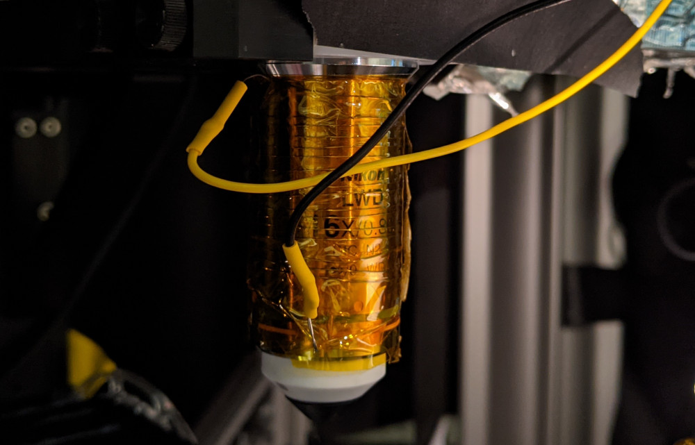
First, I like this job and what it entails: working with technology, building microscopes, working with animals, coding, analyzing data, and exploring new things every week. If you are familiar with this blog, you probably know how much I like these aspects of my work.

Second, with my research I want to contribute to the basic knowledge about the brain within the science community. I believe that this deepened basic understanding of the brain will ultimately have positive impact on our society, how we see ourselves and how we treat our own and other minds during health and disease. In this line of thought, I see myself as a servant to the public.

Third, and this is the focus of today’s blog post, doing research in neuroscience also enables me to increase and improve my own understanding of the cellular events in the brain, of thought processes, and of life in general. This is what drew me to science in the beginning.

In contrast to this last point, the work as a researcher embedded into the science machinery of the 21st century tends to be focused on something else, and for understandable reasons. Most of the daily work of scientists is focused on making discoveries, on having impact, and on being seen as successful. It almost seems a natural idea to believe that making discoveries is the same as better understanding the brain. And although discoveries might be the best way to increase the overall insight into the brain for humanity, it might not be the best way to increase your own understanding of the brain.

2. Understanding by reading from others (“passive” research)

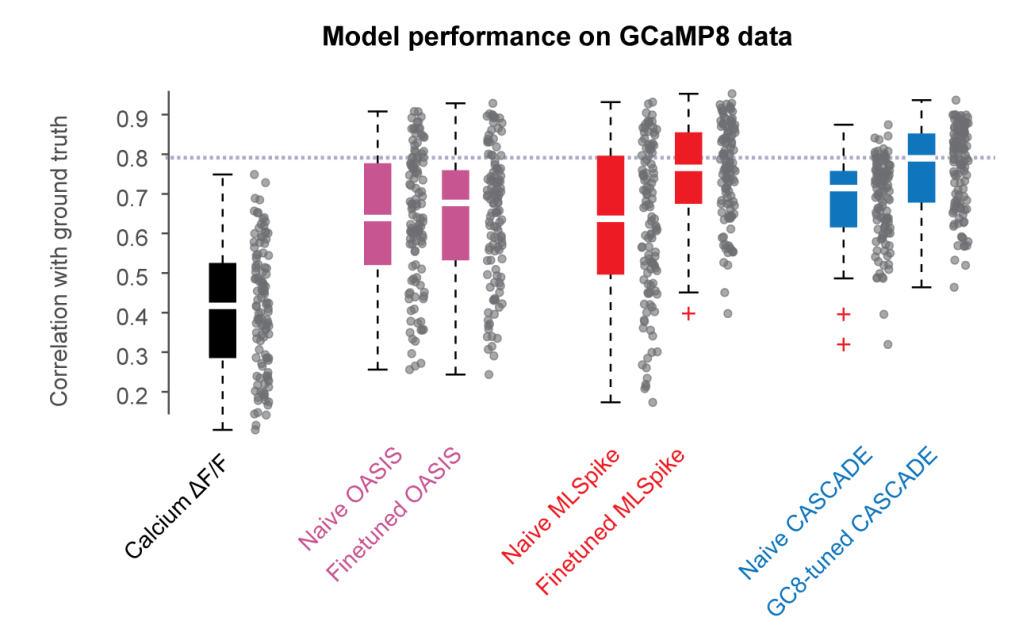
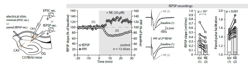
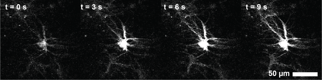
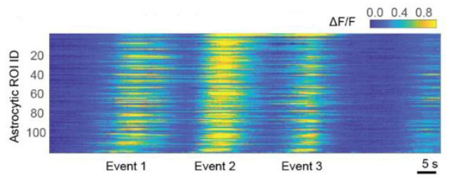
One of the tasks that kept me most busy in early 2024 was the final preparations for our publication on centripetal propagation of calcium signals in astrocytes. I still believe that this is my most important contribution to science so far, and I do think that I learnt much during this research project. However, the final steps of publication consisted of rather tedious interactions with copy editors, formatting of figures and file types, preparing journal cover suggestions, as well as advertisement of the work through discussions, talks or public announcements. All of this may be helpful for my career and useful for the potential audience, and can be fun as well, but certainly does not advance my own understanding of the brain. I felt as though I was treading water – being very busy and working hard, yet at the same time, I got the impression that I had temporarily lost touch with the heart of research.

At the same time, I had to step in on short notice to give a lecture to medical students about the motor system, covering cortex, basal ganglia, cerebellum and brainstem. Since I didn’t find the existing lecture materials fully satisfying, I began researching the topic myself. Coming from physics and having been interested in the principles of neuroscience like the dynamics of recurrent networks or principles of dendritic integration rather than in the anatomical details, I had never fully had a firm grasp of the motor system. Now, I was forced to understand the connections between the motor cortex, cerebellum, and basal ganglia, and their effect on brainstem and spinal cord, in just a few days. What role do the “indirect” and “direct” pathway play in the striatum, and how are they influenced by dopamine? What is the opinion of current research about these established ideas? What role does the cerebellum play? How should we treat David Marr’s idea of the cerebellum? What is currently known about the plasticity of Purkinje cells in the cerebellum? My understanding of these topics had been superficial at best. The challenge of delivering a two-hour lecture on this topic – and being able to answer any question from students – forced me to seriously think about these topics.

After an intense weekend that had been full of struggles, textbooks and review papers, not only had I prepared an acceptable lecture, but I had also made real progress in my personal understanding of how the brain works. It wasn’t directly relevant to my own research, but over the following months, I noticed that far more studies from the field of motor systems suddenly caught my attention – because now I understood better what they were about. Retrospectively, I could now also better understand the work on the brain stem done in the neighboring lab of Silvia Arber during my PhD.

Therefore, the most important progress in my understanding of the brain during this time in early 2024 didn’t come from my own active research or from a conference where I could catch up on the latest developments. Instead, it came from a weekend when I was forced to dive into a topic slightly outside of my comfort zone. Let’s call this “passive” research, as it did not involve my own lab activities but ‘only’ researching the conclusion from other scientists.

If I wanted to really understand the brain, wouldn’t it make sense to work this way more often? That is, instead of spending five years applying my time and expertise on a narrowly defined scientific question, shouldn’t I first aim to better comprehend the available knowledge?

3. The limitations of a “passive” research to understanding the brain

A few years ago (around 2007-2009), I had already tried to understand the brain in such a “passive” way: by systematically absorbing and mapping out the existing knowledge, while being myself not yet an active researcher. At the time, I was in the middle of my physics studies. Physics itself wasn’t my main interest but rather a means to learn the methods and ways of thinking that are necessary to penetrate neuroscience and ultimately understand the brain. At the same time, however, I realized that I lacked some basic knowledge in neuroscience. For example, I had some notions about the different brain regions, but these notions were very vague and consisted of not much more than names.

To change this lack of knowledge, I started a project that I called “The brain on A4” (A4 is a paper page format similar to the US letter). The idea was to search the literature for a given brain region, summarize the findings, and condense them onto a single A4 page. My vision was to eventually wallpaper my room with these 100 A4 pages so that the summarized facts and essential insights about all relevant brain regions would always be present as anchor points for my thought processes. This way, they would gradually sink into my mind and provide the foundation for a deeper understanding through reflection and the integration of new thoughts.

For illustration, here are two pages of the “Brain on A4” project, written in German (with a few French textbook excerpts included since I was studying also at a French university then).

In short, the idea didn’t work. Using this approach, I covered some brain regions, and when I read through these A4 drafts today, they don’t seem completely off base. But the concepts that are now familiar to me and connected to other topics had only vague meanings back then when I copied them from Wikipedia, Scholarpedia or review articles that took me several days to go through. I could recall the keywords and talk about them, but I couldn’t truly grasp them when I put myself to the test.

Why? Because knowledge must grow organically. It needs both contextual embedding and emotional anchorage. This embedding can be a discussion partner, or a project where this knowledge is applied or tested, or, at the minimum, it can be the exam at the end of the semester where the knowledge is finally “applied”.

In addition, I was also lacking the toolset to probe the knowledge. Different from maths, physics or foreign languages, the knowledge about the brain comes in vague and confusing sentences that are difficult to evaluate. That is, for most of the statements of the brain, it is difficult to say whether it is indeed true or what it means. The equation for potential energy E = m·g·h can fully understood by derivations or examples. On the other hand, the statement “The major input to the hippocampus is through the entorhinal cortex” (source) only makes sense (if at all) when the entorhinal cortex is well-understood (which is not the case). In addition, neuroscientific publications are full of wrong conclusions and overinterpretations. For example, if I randomly take the latest article about neuroscience published in Nature, I get this News article of a research article by Chang et al. . The main finding of the study is indeed interesting and worthwhile reporting: recent memories are replayed and therefore consolidated during special sleep phases of mice where the pupil is particularly small. The News article, however, stresses that this segregation of recent memories into distinct phases may prevent an effect called catastrophic forgetting, when existing memories are overwritten because they use the same synapses. This interpretation, however, is quite misleading. Catastrophic forgetting and the finding of this study are vaguely connected but not closely linked, which becomes quite clear after reading the wikipedia page on catastrophic forgetting. As a lay person, it is almost impossible to understand that this tiny part of the discussion, which prominently featured in the subheadings of the News article, is only a vague connection that does not really reflect the core experimental findings of the study.

Similarly, when I made the A4-summaries, I meticulously listed the inputs and outputs of brain regions. But what could I make out of the fact that the basal ganglia receives input from cortex, substantia nigra, raphe and formatio reticularis (as in my notes above), if all of those brain areas were similarly defined as receivers of input from many other areas? Back then in 2008, I wrote about the cortico-thalamic-basal ganglia loops and how they enable gating (see screenshot above), but only when I worked through the details again with a broader knowledge base 16 years later, I managed to see the context where I could embed the facts and make them stick in my memory. And it took me this many years working in neuroscience to slowly grow this context.

4. The limitation of a systematic approach to understanding the brain

A second reason why this approach for mapping the brain to A4 pages didn’t work may have been its systematic nature. A systematic approach is often useful, especially when coordinating with collaborators, or when orchestrating a larger project. However, I’ve come to believe that a more organic – or even chaotic – approach can be more effective, especially when it comes to understanding something. A systematic approach assumes that you can determine in advance what needs to be done, in order to faithfully follow this structure afterwards. For the A4 project, the systematic structure was the division into “brain regions.” Of course, the brain can not be understood by just listing the properties of brain regions; many important concepts take place on a different level, between brain regions, or on the cellular level. I noticed the limitations of my approach myself soon enough and added A4 pages on other topics that I deemed relevant like “energy supply to the brain” and “comparison with information processing in computers.” The project lost its structure, for good reason. And soon after, before the structure became completely chaotic, I abandoned the project entirely.

One thing that I learnt from this failure is how a systematic approach can sometimes hinder understanding. In formal education, this truth is often hidden because curricula and instructors provide the structuring of knowledge already. But when it comes to acquiring new knowledge and insight, rather than merely processing and assembling pre-existing knowledge, this systematic approach must be continuously interrupted and re-invented to enable real progress. When I first heard about the hermeneutic circle, invented by hermeneutics (the science of understanding a text), I had the impression that this concept was an accurate description of the process of understanding. Following the hermeneutic circle, deeper understanding is approached not on a direct path but iteratively, by drawing circles around the object of understanding, maybe constructing a web of context and possibly an eventual path towards the goal. In this picture, the process of understanding is diffuse and unguided, and is corrected only occasionally by counscious deliberation and a more systematic mind. As a consequence, the object of interest can only be treated and laid down systematically once its understanding has been reached, but not on the way to this point.

5. The limitation of a non-systemic approach to understanding the brain

However, the unsystematic approach to understanding the brain has a major drawback: you lose the sense of your own progress, and you lose the overview of the whole. Often, progress is incremental and, over years, so slow that you hardly notice you’ve learned something new – leading to a lack of satisfaction. And, even more importantly, you lose the big picture.

This may also be one of the greatest barriers to understanding the brain: the possible inability of our minds to comprehend the big picture of such a complex system where different scales are so intricately intertwined. A few years ago, I wrote a blog post about this topic (“Entanglement of temporal and spatial scales in the brain, but not in the mind”), which I still find relevant today. Can we, as humans with limited information-processing capacity and working memory, understand a complex system? Or more precisely: what level of understanding is possible with our own working tool – the brain -, and what kind of understanding lies beyond our reach?

Recently, Mark Humphries wrote a blog post to address a similar question. He speculated that the synthesis and understanding of scientific findings may, in the future, no longer be carried out by humans but by machines – for example, by a large language model or a machine agent tasked with understanding the brain. Personally, I find this scenario plausible but not desirable. An understanding of the brain by an artificial agent that is beyond my own ability may be practically useful, but it doesn’t satisfy my scientific curiosity. Therefore, I believe that we should focus on how to support our own understanding in its chaotic nature and, perhaps retrospectively, wrest structure and meaning from this chaos. How? By writing for yourself.

6. The importance of writing things up for yourself

As I mentioned earlier, I believe that understanding the brain is a chaotic and iterative process that does not proceed systematically or in a predictable trajectory. Instead, it involves trying out different approaches and constantly adopting new perspectives. For me, these approaches include reading textbooks and preparing lectures; reading and summarizing current papers; and conducting my own “active” research in the lab and in silico.

During this process, I found that shifting one’s perspective can be particularly helpful in gaining a better understanding. To gain such new perspectives, I regularly read open reviews, which often present a picture different from the scientific articles themselves. Or, I like to explore new, ambitious formats that shake off the dust of the traditional publication system and attempt to take a more naive view of specific research topics. A venue that is still fresh in spirit and that I can recommend for this purpose is thetransmitter.org.

However, the best method to adopt knowledge and integrate it into one’s own world model is by processing the knowledge in an active manner. The two methods I find most useful are mind maps and writing. Usually, I use mind maps when I’m completely confused, either about the direction of a project, or about my approach to neuroscience in general. Usually, I just start with a single word in the center of a paper within a circle and then add thoughts in an associative manner for 20-30 minutes. The result of this process is not necessarily useful for others. However, seeing the keywords laid out before me, I can often see the missing links or identify things that should be grouped together, or grouped differently.

Below is an example of a such mind-map. I drew this map in 2016 a bit more than two years into my PhD, at a stage where I was quite struggling to shape my PhD project. Unlike most of my mind maps which are hand-drawn and therefore almost illegible to others, this one was drawn on a computer (in adobe illustrator, to play around with the program). I was brain-storming about the role of oscillations in the olfactory bulb of zebrafish (check out this paper if you’re interested). Although I did not follow up on this project, some of the ideas are clearly predecessors of analyses in my main PhD paper on the olfactory cortex homolog in zebrafish. The mind-map is basically a loosely connected assembly of concepts and ideas that had been living in my thoughts, often inspired by some reading of computational neuroscience papers or by discussions with Rainer Friedrich, my PhD supervisor. I used this map to visualize, re-group and connect these ideas:

The second method is writing, and I believe that it is the only true method to really understand something. In contrast to reading, writing is an active process, and so much more powerful in embedding and anchoring knowledge in your own mind. You may have heard of the illusion of explanatory depth, the tendency of our brain to trick us into thinking we understand something simply because we’ve heard about it or can name it. Only when we attempt to explain or describe a concept, we realize how superficial our thoughts were and how shaky our mental models really are. Writing is a method for systematically destroying these ill-founded mental structures. (Expressing an idea in mathematical or algorithmic terms is even more precise and therefore even better for this purpose!) When we have destroyed such an idea, we shouldn’t mourn the loss of a seemingly brilliant concept but instead celebrate the progress we’ve made in refining our understanding.

In addition, writing has always been a form of storytelling. By putting our understanding of the brain into words – even if those words are initially fragmented, scattered, and contradictory – writing seeks to find meaning, identify patterns, and embed details into a larger whole. With a bit of practice, writing does all of this for you.

Importantly, I’m not talking about writing papers or grant proposals here. In those cases, you have a clear audience in mind (editors or reviewers) and eventually tailor your writing to meet their expectations. And you will be happy and satisfied when you produce something that meets the standards for publication. Instead, I’m talking about writing for oneself. This mode of writing confronts your own critical voice and follows ideas without regard for how the text would look like. And I believe that this way of writing, which is not directly rewarded by supervisors or reviewers, is the most useful in the long run.

I believe that many researchers in neuroscience (and maybe you as a reader) initially started to work as neuroscientists not because they wanted to be famous or successful or well-known but because they wanted to understand how the brain works. So if you want to take this seriously, write for yourself.

Posted in Data analysis, Neuronal activity, neuroscience, Reviews | Tagged brain, neuroscience, research, science, theoretical neuroscience, writing | 9 Comments

A resource paper for building two-photon microscopes

Posted on September 28, 2024 by P.T.R. Rupprecht

Building microscopes in the lab is a skill that is rarely taught at university. It is no coincidence that most people who have learnt to build microscopes have done so in the lab from other researchers or engineers. Usually, one needs to be lucky to find pieces of knowledge in random papers, in discussions with experts, or when browsing blogs like the one you’re currently reading. A part of the problem is that most papers that describe the novel design and construction of microscopes are often challenging to translate into practice even for experts because they describe the ideas and concepts and do rarely provide precise assembly instructions together with the rationale behind.

In their manuscript on An open-source two-photon microscope for teaching and research by Schottdorf et al., the authors go a different route. Instead of presenting a novel microscope design that shall be used for future experiments, they describe the rationale and principles behind a microscope design that was already used, tested and refined over many years in a very successful systems neuroscience lab.

Assembly of lens groups for tube lens and scan lens. From (Schottdorf et al, 2024), under CC BY 4.0 license (Supplementary Material, Figure 8).

The paper includes many interesting and useful pieces of knowledge. Among those, I would like to highlight only a few:

The assembly instructions and rationale for a custom scan lens and tube lens based on off-the-shelf components (see the Results section, but also the Discussion with comments on ideas from astronomy and photography).

A similar design suggestion and analysis for the detection path.

A discussion why an axial FWHM of 5 μm is, in the view of the authors, a pragmatic compromise for in vivo-imaging with movement artifacts.

The interesting side-note that ±28 V instead of ±24 power supply specifications are advantageous for galvo scanner performance.

The measurement of the dispersion for this specific two-photon system, which can be considered typical for two-photon microscopes (approx. -20000 fs²).

In addition, the manuscript comes with a very nice documentation on Github that includes a detailed assembly protocol, a list of parts including prices of laser, objective, shutter, power meter, PMTs, etc.

Altogether, a great resource that is definitely worth a look.

Posted in Calcium Imaging, Imaging, Microscopy, neuroscience | Tagged Calcium Imaging, Microscopy, neuroscience, papers, photons, Scanning, science | 1 Comment

Spike inference with GCaMP8: new pretrained models available

Posted on August 22, 2024 by P.T.R. Rupprecht

Calcium imaging is only an indirect readout of neuronal activity via fluorescence signals. To estimate the true underlying firing rates of these neurons, methods for “spike inference” have been developed. They are useful to denoise calcium imaging data and make them more interpretable. A few years ago, I developed CASCADE, a supervised method for spike inference based on deep networks. I have been been updating and maintaining CASCADE ever since, and this maintenance work has been a starting point for several collaborations and friendly interactions during the last years (for example, check out this recent preprint on spike inference from spinal cord neurons).

Originally, the CASCADE algorithm was trained on a ground truth database that consisted primarily of recordings with GCaMP6. However, how will the algorithm perform on new indicators like GCaMP8, with its much faster rise times? To address this question, I now trained CASCADE models on GCaMP8 ground truth and evaluated whether these models performed better than previous models. The short answer is – the retrained models performed clearly better:

I’m currently in the process of dissecting this improvement: Is it due to differences in rise times, different non-linearities or other differing properties of the two indicator families? The results of these analyses turned out to be more fascinating than I expected and therefore take more time to understand and analyze, but I’m planning to have this analysis written up within the next 3-6 months.

In the meantime, however, feel already free to use the new CASCADE models specifically trained with and for GCaMP8 – they really make predictions better! (And please only apply these models to GCaMP8 data; the previous models are still better for anything with GCaMP6!)

You will find the new models for CASCADE as usual in the list of available pretrained models. For example, instead of the GCaMP6-trained model Global_EXC_30Hz_smoothing25ms, indicate the GCaMP8-trained model GC8_EXC_30Hz_smoothing25ms_high_noise to infer spike rates with the predict() function of CASCADE.

A technical note: These models are pretrained on all available GCaMP8-ground truth, mixing together GCaMP8f, GCaMP8m and GCaMP8s. This procedure results in more robust models due to the larger ground truth database, but absolute inferred spike rates are slightly biased due to the different spike-event fluorescence amplitudes for the three indicators (-30% underestimate for GCaMP8f and GCaMP8m, +60% overestimate for GCaMP8s). In the near future, CASCADE will also include models specific for each of those indicators. These models will probably be slightly less robust but will provide less biased spike rates. However, if you are not specifically interested in very precise absolute spike rates, I would for now recommend the general GCaMP8 models that are already available. They are not only robust and very powerful but also provide a good rough estimate of absolute spike rates.

Update 2024-09-19: Models pretrained with specific indicators (e.g., GC8s_EXC_30Hz_smoothing25ms_high_noise for GCaMP8s) are now available online. Check out the full list of models via the Cascade code or via this continuously updated list on Github.

Update 2025-03-11: A preprint describing the analyses, the pretrained models and their applications to GCaMP8 is now on bioRixv: https://www.biorxiv.org/content/10.1101/2025.03.03.641129.

If you have questions, please reach out via comments on the blog, issues on Github or via email!

Posted in Calcium Imaging, Data analysis, Imaging, machine learning, Network analysis, Neuronal activity | Tagged Calcium Imaging, Data analysis, deep learning, electrophysiology, Microscopy | 4 Comments

How to do science according to Ardem Patapoutian

Posted on August 19, 2024 by P.T.R. Rupprecht

Ardem Patapoutian is a neuroscientist who works on the molecular basis of sensation via mechanosensitive ion channels. In 2021, he was one of the recipients of the Nobel prize, at a relatively young age. He has since used his influence among scientists to speak out for improving academia for both research and the humans who do the research.

In a post on Twitter, he compiled a list of 13 rules on how to do science. I strongly agreed with some aspects, disagreed with others (after all, Ardem is a scientist in a slightly different field), and felt inspired to share some thoughts about his list. I’m writing these comments also because I’m curious what I will think about my current ideas in 10 or 20 years from now. Here’s the list:

1. Don’t be too busy (Rule #1: No excuses. If you’re too busy, you’re not being creative).

I’d subscribe to this statement 100%.

As a PhD student, I had only few fixed responsibilities. Every couple of months, I started a new side-project, learned a completely new experimental technique, a new programming language, read about a new field of computational neuroscience, etc. 7 years ago, I gave an interview about this creative process for my science. I believe that these deep dives into unknown territory are necessary for creativity. Creativity is often a combination of two influences from two different fields; in the simplest case, it’s just the application of a certain domain to another – let’s say, the use of a fancy cooking technique for the improvement of an immunohistochemistry method. Such a knowledge transfer requires not only focused work on the target method (immunohistochemistry), but also a deep knowledge about the other field (fancy cooking), which requires time, an exploratory spirit – and an appreciation for the fact that time spent understanding one domian can always be beneficial for another domain.

I noticed for myself that the available time that I have for such digressions became less once I became a PI, and it will become worse over time in the future. But I hope to maintain conditions in the future that won’t prevent me from staying creative!

2. Learn to say no (related to #1).

That’s a very commonly given advice, but few people seem to follow it. “Saying no” is not only about focusing on one’s own projects and tasks, but also about saying no to the inner voices and the peer pressure. You need to publish in Nature. No, you don’t; don’t lose yourself while trying. You need to finish your PhD with 30. No, everybody at their own pace! You need to have >3 PhD students. No, one may be just enough for some situations. You need to become a professor within 5 years. No, you don’t. Life outside academia has many things to offer.

For some people, learning “no” only seems applicable to requests from other people. But learning to say “no” to the internal voices – which are often only the internalized voices of other people, be it peers, parents or professors – can be even more important to free the mental resources for doing creative work and for doing real science.

3. What question to ask: Find the biggest unanswered question that can be approached in the next 5-10 years.

I don’t fully agree with that one for my field of science. In basic systems neuroscience, the relevant question is “how does the brain work”, and it cannot be approached within 5-10 years. In the meantime, from my own perspective, it seems to make more sense to find small islands of mechnistic understanding and curious observations (for example, I could pick behavioral timescale synaptic plasticity in hippocampal neurons or centripetal integration in astrocytes as starting point phenomena) and continue to work from there bit by bit, even though it’s not yet clear how these questions can be answered within 10 years.

4. Science communication: When you talk about your work, always start by stating what the important open question is (this is fundamental, but very few do it; related to #3).

That’s good advice! I should do that more often.

5. Prioritize: Know when to quit a project (as important as coming up with new ideas).

Very good advice again.

I think it is very beneficial to invest a lot of energy trying to kill a project as early as possible. For example, trying to find a critical flaw in a conceptual idea before implementing it in a tedious series of experiments, and then realizing that the data cannot be analyzed properly.

For example, a typical situation at the beginning of an experimental systems neuroscience project is the design of a behavioral task for an animal. Will it be possible to extract the desired mental states from the acquired data, or will these states be confounded by movement or arousal of the animal? These are questions that need to be considered before, not after the experiment.

It happened to me already 3 times that I stopped my main scientific project (1x during my PhD, 1x during my postdoc, 1x as junior PI) because I convinced myself by theoretical arguments or by some analyses that it would not work out. And it happens much more often for smaller project.

6. Change fields when the open questions are no longer interesting: Being from a different field allows you to look at problems with a fresh perspective.

I’m very skeptical about this piece of advice. Maybe I’ll think differently in 20 years. But at the moment, I have the impression that those who stay in a field and try to figure out the little details are my real scientific heros. If you’ve found a real effect, you should go for it fully and not drop it for the newest hot stuff. Otherwise, one risks joining a new field where the open questions only seem interesting from outside, the typical “hype train”.

7. Ask for help – don’t reinvent the wheel.

As somebody who built several microscopes and data analysis pipelines from scratch, I can agree only very reluctantly. I learnt so much from reinventing these wheels! And I would be a much worse scientist without.

I still remember my first year of physics studies, when I did not know of any sort of theoretical neuroscience. Back then, I tried to develop a weird form of math that can deal with neuronal connectivity and dynamics. Only a year later or two, I stumbled across Dayan & Abbott’s famous Theoretical Neuroscience and learned that matrix algebra is a great and existing tool for that. But I still wonder what kind of math I would have come up with if I’d been more gifted for it and if I’d had more time without Dayan & Abbott.

However, I also noticed that several extremely skilled scientist-tinkerers like Jakob Voigt and Spencer Smith (I was unable to find his blog post on this topic) turned into advocates of professional infrastructures later during their careers, advocating against the repeated reinvention wheels.

I still cannot decide whether the established black box button-press infractructure are more error-prone, or the code written from scratch by a very smart PhD student. From the perspective of a PhD student, it is probably better to write and build everything from scratch, because you learn more and know what is going on. From the perspective of the PhD student’s supervisor, however, it is better if an existing and tested infrastructure is used, because otherwise there is no efficient way to make sure that the results obtained by the PhD student are valid. Maybe these two different perspective are also the reason why some people change their mind once they are professors.

8. Don’t listen to advice if it doesn’t make sense to you (this does not contradict #7).

No strong opinion on that.

9. Hire people who are smart, efficient, and kind (don’t forget about “kind”).

Agree. Even more important: As a PhD student, join a lab with a smart, efficient and kind PI (don’t forget about “kind”).

10. Champion the underprivileged.

Agree.

11. Collaborate with people with very different training and experience.

I have a hard time agreeing with this rule. My best collaborations have been with people who were technically stronger than me. Collaborations with people who have only limited understanding and, in particular, limited appreciation for the skills that I bring into a collaboration, can be quite painful. But maybe I will judge collaborations from an entirely new angle in 10 years.

12. Cultivate friends who tell you when you are wrong.

I noticed that senior PIs often do not have anybody (not a single person!) who tells them with all honesty when they are wrong. If such a condition is combined with a narcisstic personality of the senior PI, things can become really bad and embarrasing. I do not yet know how exactly to prevent this from happening, because it seems to happen to the best scientists, and it seems particulary common for men (less so for women according to my observations).

13. Don’t forget why you got into this business in the first place: Science is fun. Minimize the noise that causes anxiety.

I also think that reduction of anxiety is indeed important (related to #1 and #2). But I don’t have a recipe on how to reach such a state. From my own and very limited experience as an observer, the level of anxiety seems to be relatively stable for a given person within academia, independent of the position. I happen to be one of those persons who are not very anxious in general. The reason for this lack of anxiety is maybe that I’m not afraid of leaving academia, because I’m sure I would find another interesting job as well, and because my family does not have any ties with academia. But first of all, it’s probably a personality trait which I owe primarily to my genes and to my parents – and I’m grateful for that!

Posted in neuroscience, Uncategorized | Leave a comment

On the night train to FENS in Vienna

Posted on July 25, 2024 by P.T.R. Rupprecht

The FENS is the biggest neuroscientific conference in Europe. It is 5 days long and is attended by 5’000-10’000 participants. This year, the conference took place in Austria’s capital, Vienna, roughly 600 km from my current workplace in Zürich. Of course, there are regular and cheap flight between the two cities; however, there are good reasons why to use other means of transportation instead (check out Anne Urai‘s work): busses, regular trains, and night trains. In this blog post, I will share my impression what it is like to take a night train in Europe and why it is a great option for some (but not for everybody).

What’s special about night trains?

Night trains (also called sleeper cars) typically cover longer distances than regular trains. Traditionally, they tried to offer more comfort for an over-night stay, like comfortable beds, additional cars with proper restaurants and bars, or at least a breakfast served at your seat. Especially in times when trains were slower and airplanes not available, night trains were one of the more comfortable options to make a long trip enjoyable. I was surprised to find out that some of the earliest night trains were actually operated in the USA! However, the probably most famous examples of night trains traverse the Eurasian continent. For example, the Transiberian Railway, which extends from the Western to the Eastern Border of Russia; or the Orient Express, which passes through a large part of Europe from Paris to Istanbul.

Seating carriages, sleeper’s carriages and things between

In most night trains that I know, there are three different carriages. First, the cheaper carriages where you stay on a seat over night. Sometimes, these seats can be pulled out and converted into an improvised bed. Second, the couchette, which offers bunk beds, usually with 4 or 6 beds within one compartment, with 2 or 3 stories on the left and the right. And finally, a more spacious and more private sleeper compartment, with typically 1 to 3 beds. It is also possible, for an additional fee, to reserve a sleeper compartment for oneself, for a couple or a family. The prices are moderate when booked much in advance; for example, I paid <150 Euros for the round trip from Zürich to Vienna. However, one must also state that (and wonder why) a cheap flight is not much more expensive than that.

The current state of night trains in Europe

Unfortunately, night trains have been on the decline for several decades in Western Europe. With more and more cheap flights or good high-speed train connections between many European cities, the operation of the slower night trains became less interesting for railway companies, and investments stalled. Around 2020, some governments in central Europe tried to countersteer this decline by pushing for a stronger network of night trains. But it will still take several years until these efforts will show some effect, and the success is not a given.

The re-growing interest for night trains didn’t come out of nowhere. With the public opinion looking more skeptically at short-distance intracontinental airplane flights, night trains in Europe became increasingly popular, in particular after the pandemic, as a CO2-friendly option for long distance-traveling. However, the infrastructure could not really hold up to the increasing interest. Most importantly, the fleet of trains was both too old and too small for the rising demand. The companies responded by using their trains at maximum capacity; therefore, if a carriage broke down (which was not unlikely due to their old age and the scarcity of spare parts), often there was no replacement carriage, and the passengers who were supposed to calmly sleep in a reserved bed were regrouped into an overcrowded seating carriage. Addtionally, the infrastructure inside of the carriages, like toilets, bed lights, etc. is often rather old and not always in a good state – far from the luxury atmosphere associated with, e.g., the Orient Express! Moreover, night trains are often delayed by one or several hours, especially on high-demand routes such as Zürich-Amsterdam.

In summary, one needs to face the fact that night trains are currently not as reliable and not as comfortable as they should be in order to make this mode of traveling attractive for a broader audience. It is likely that the situation will improve during the next years, with more modern cars being produced, replacing and supporting the existing fleets, and making night trains in Europe again more reliable and also luxurious. I have the impression that the companies have already taken some good first steps towards such an improved scenario, because when I took the night train to Vienna, the train was purposefully underbooked, most likely to prevent major problems in case a carriage would break down. But let’s see what the next years and decades will bring.

My own experience has so far been limited to night trains operated by the German-speaking railway companies, with the Austrian railway company ÖBB being at the heart of it. However, there are other night trains as well. For example, it’s possible to go from Milano in Northern Italy to Sicily within a long night, passing not only the largest part of Italy, but also the Mediterranean Sea with a train ferry (!). So if you’re planning your next series of Summer conferences to attend across Europe, maybe you can connect the conferences with an adventurous night train trip?

Screenshot from https://back-on-track.eu/night-train-map/, CC-BY-NC Juri Maier / Back-on-Track.eu .

Traveling from Zürich to Vienna with the night train

The conference in Vienna started on Tuesday, June 25th, with a workshop on closed-loop neuroscience that I wanted to attend (and I was particularly impressed by the cool work from Valerie Ego-Stengel’s lab). I worked normally in Zurich on Monday and went directly from work to the main train station, where the night train departed at 8.40 pm. With me, the luggage for a Summer’s week and a big poster roll.

My train was, to be fair, quite old. I had booked a sleeper’s bunk bed in a 6-person compartment but the middle beds on each side were not used, as you can see below. You can also guess from the first picture and see from the second picture that there was not a lot of space between my bunk bed and the ceiling. It was enough to sit on the bed and work, but barely.

When I entered the compartment, I realized that I would share it with an elderly Indian couple, who were, while the train was still waiting in the station, accompanied by several family members. The couple was from Vienna and had attended a wedding in Switzerland. As most people in night trains, they had little experience with the night train experience. What are the rules? What bed should you take? When will the lights be turned off? Where are the electric plugs? Is there wifi? (Usually, there is none.) Will I be woken up in the morning? I could see the anxiety and the adventure in their eyes, and they were grateful that I could help out with some of their simplest questions.

We had a pleasant discussion about their lifes in Vienna, but after a short time, we decided to go to bed. I went up to my bed and spent an hour or two going through the scientific abstracts of the conference to figure out the best trajectory for the next days. Around midnight, I went to sleep. It turned out that this particular car and this particular bed was not perfect for me – the bed measured almost exactly 180 cm, which is a few cm too short for my height. I noticed that the lower beds were slightly longer, from which I benefitted gladly when I took the train back a few days later.

Usually, I can sleep pretty well in night trains. I like the rhythmic rattling of the train wheels, it even helps me fall asleep (to the extent that I find it difficult to sleep when the train is not rolling but standing still in the middle of the night for an hour!). It’s a pleasant feeling to know that the goal is coming closer by itself while I do nothing but sleep.

This time, however, I was a bit unlucky. My two cabin mates were very friendly when awake, but rather annoying during sleep. The woman was snoring in an irregular way that I found difficult to deal with, while her husband was occasionally speaking or shouting in his sleep with an agitated voice. Not my best night train night so far! I heard later that a colleague of mine who also took the night train to FENS was much luckier, sharing the cabin with other attendants of the FENS conference and having a good time during the evening and night.

In any case, the train arrived at 6.34 am in Vienna, perfectly on time. The breakfast in the train had not been exceptional (which is unfortunately the rule rather than the exception according to my experience). Therefore, I benefitted from the great Viennese baking culture and got a very decent breakfast at a price that seemed so much more affordable as I was directly coming from Switzerland…

After the 5-day conference, which was a pleasant mix of meeting old friends and meeting people for the first time I knew from Twitter, from collaborations or from eMail exchanges, interspersed with some interesting pieces of neuroscience, I spent another day with a good old friend of mine who happens to live in Vienna, before I took the train back to Zürich. My plan was to take the night train on Sunday just after 11 pm, to arrive on Monday morning in Zürich and go directly to work. Maybe an ambitious plan, but it worked out well. During the last hour before my train departed, I waited at the train station in Vienna, with the vibrant atmosphere of Summer still around me. Due to the European soccer championship, one of the games was publicly displayed on a huge screen just in front of the station, and a Spanish crowd cheered every time their team scored a goal.

Back on the train, I entered the compartment that was already occupied by one woman, sleeping in one of the beds, hidden below the blanket. I tried to do my best not to wake her up and took over the bed on the left.

I wrote a few notes on my laptop to record the recently passed very eventful and inspiring days, and then fell asleep.

I woke up in the early morning around 6.30 am. With joy, I noticed that we were passing by Lake Walenstadt, a beautiful lake in the East of Switzerland, and already quite close to Zürich. Through their diffuse reflection, the grey and white clouds created a beautiful metallic shimmer in the water, and I sat there, looking out of the window, being happy.

Soon after, we passed by Lake Zürich, and when I arrived at Zürich main station, I had my breakfast with delicious Viennese pastries before I went to work. A very efficient way of traveling!

Why you should (not) take the night train

It should have become clear now that night trains in their current state are not for everybody. The comfort is too low and the prices are a bit too high, and delays too frequent. But still … I would recommend this experience to anybody who is not afraid of it and can manage to sleep in such a context. It’s not only about avoiding airplanes, but also about embracing the adventure that is much more palpable for the night train experience compared to airplane flights. The sense of adventure not only makes the travel special but also bonds the travellers within one compartment to each other more easily. A great opportunity to meet with people from outside your social circles!

The probably most famous night train, the Orient Express, has long been associated with an atmosphere of both luxury and adventure. And both aspects are reflected by its prominent occurrence in works of fiction, ranging from Agatha Christie’s famous novel The murder on the Orient Express to the most recent Mission Impossible movie. Nowadays, it is mostly the atmosphere of adventure which still remains part of the night train experience. Almost 20 years ago, I was deeply fascinated by the novel Night Train to Lisbon. In this book, the daily life of a high school teacher transitions to a philosophical and linguistic adventure within a single night: in the night train from Bern to Lisbon. I still believe that this is the essence that is the most attractive aspect of night trains: the vague promise of adventure, a memorable night and a new world that opens up to the awakening senses on the morning of the next day.

Posted in Uncategorized | Leave a comment

A collaborative review on error signals in predictive processing

Posted on July 23, 2024 by P.T.R. Rupprecht

Predictive processing is one of the most influential ideas from computational neuroscience for the experimental neurosciences. However, definitions of predictive processing vary broadly, to the extent that “predictive coding” is used sometimes in a very narrow sense (there are specific cell types for negative or positive expectation errors) or in a very broad sense (anything related to error signals or expectation mismatch is predictive processing).

Jerome Lecoq now started the great initiative to write a review about error signals for predictive processing, but in a very collaborative manner. He invited anybody interested to join the writing of the review.

I think that this way of writing a collaborative and open review is a great idea, even though it might be difficult to reconcile all the different opinions! This link will lead you to the Google document with the main text and with the instructions on how to contribute. And if you don’t feel like you want to contribute, it is at least a useful opportunity to learn about the current opinions in the field and how people agree or disagree about the interpretation of predictive coding, error signals and the literature that covers both. Take a look!

Posted in Calcium Imaging, Data analysis, machine learning, Neuronal activity, neuroscience, Uncategorized | Tagged Data analysis, deep learning, machine learning, theoretical neuroscience | Leave a comment

Four interesting papers on astrocyte physiology

Posted on July 8, 2024 by P.T.R. Rupprecht

During the last years, I have been working to understand not only neurons but also astrocytes and their role in the brain. The mode of action of astrocytes is dominated by a diversity of potential molecules and pathways involved and an almost equal diversity of opinions about what is the most important pathway. It is however clear that astrocytes sense many input molecules; there is a consensus that calcium might be a key player for intracellular signaling in astrocytes; and there are quite opposing views about the most relevant output pathways of astrocytes. In the following, I will discuss four recent papers on how astrocytes interact with neurons (and with blood vessels).

Norepinephrine Signals Through Astrocytes To Modulate Synapses

Do neuromodulators like noradrenaline act directly upon neurons, or are these effects mediated by, for example, astrocytes? In reality, it is not black or white, but an increasing number of scientists have acknowledged the potential big role played by astrocytes as intermediates (see e.g. Murphy-Royal et al. (2023)). In this study, Lefton et al. (2024) from the Papouin lab use slice physiology to carefully dissect such a signaling pathway from neuromodulators to astrocytes to neurons.

It is rare to see such consistent and convincing evidence for a complex neuromodulation signaling pathway as it is presented in a paper. To drive home the main messages, the authors apply many controls and redundant approaches from pharmacology, optogenetics. They use three different tools for astrocyte silencing (iBarks, CaleX and thapsigargin), conditional and region-specific knockouts and two-photon imaging to confirm their ideas. I think the paper is definitely worth the read. The main conclusion is that noradrenaline release in hippocampus silences pre-synapses of the CA3 -> CA1 pathway (the so-called Schaffer collaterals). This presynaptic effect is convincingly shown with several lines of evidence. The demonstrated mode of action of this pathway is the following: noradrenaline binds to alpha1-receptors of hippocampal astrocytes. Those astrocytes release ATP, which is metabolized to adenosine. Adenosine in turn binds to the adenosine A1-receptor that has been shown to locate at the CA3 -> CA1 presynapses, finally resulting in silencing of these synapses. Together, this cascade results in long-lasting synaptic depression on the timescale of minutes. Quite impressive work!

From (Lefton et al, 2024), under CC BY 4.0 license (excerpt from Fig. 1).

There are a few caveats to consider when interpreting the study. First, most of the work was done with a noradrenline concentration of 20 uM in the bath. This is relatively high, especially given previous work that showed somewhat opposite effects for sub-uM concentrations (Bacon et al., 2020). One can speculate that the physiological effect of the pathway found by Lefton et al. may therefore be weaker and, instead of fully silencing the presynaptic effects, rather tone down their relative importance compared to other inputs. The observed effect and signaling cascade is, however, interesting by itself.

Second, Lefton et al. convincingly show that the presynapses are depressed after noradrenaline release. This finding is also accurately reflected in the title. However, in some places, the finding is reframed as an “update of weights” in a non-Hebbian fashion, and “reshaping of connectivity”. This description is not wrong, but a bit misleading because these terms suggest an important role for memory and long-term potentiation, which is not how I would interpret the results. But this is just a minor detail.

Thinking about these results, I’m wondering how specific the effect is on the investigated CA3 -> CA1 synapses. It is an appealing idea to think that, e.g., synapses from entorhinal cortex (EC) onto CA1 might be less affected by this signaling pathway. This way, noradrenaline could be used to specifically reduce inputs from CA3 vs. inputs from EC. An obvious next step for a follow-up study would be to investigate the distribution of A1 receptors on different synapses, and the effect of noradrenaline via astrocytes on other projections to CA1.

Altogether, despite the caveats, this is really a nice paper, and it clearly shows the raw power of slice work when it is performed systematically and thoroughly. This work is particularly interesting as a companion paper describes a very similar pathway with noradrenaline, astrocytes and adenosine to silence not only neurons but also behavior (Chen et al., 2024).

A spatial threshold for calcium surge

Our own work has recently shown that astrocytic somata conditionally integrate calcium signals from their distal processes, and we have shown that the noradrenergic system is sufficient to trigger such a somatic integration (Rupprecht et al., 2024). In this conceptually related paper, Lines et al. (2023) from the Araque lab similarly describe conditional somatic activation of astrocytes, which they term somatic “calcium surges”. However, they use distal calcium signals rather than noradrenaline levels to explain whether these somatic calcium surges do occur or not.

Their main finding is a “spatial threshold”, i.e., a threshold of a minimum fraction of distal astrocytic processes that need to be activated in order to lead to somatic calcium surges. This is an interesting finding which they validate both in vivo and in slices in somatosensory cortex. The authors quantify that activation of >23% of the arborization results in a somatic calcium surge. Although I like the attempt to be quantitative and makes the results easier to compare to other conditions, I believe that the precise value of this threshold is a bit over-emphasized in the paper. I believe that this specific value could change quite a bit with different imaging conditions, with different analysis tools, or when assessing the calcium signals volumetrically in 3D instead of in a 2D imaging plane. However, I still like the overall approach, and I think it is quite complimentary to our approach focusing on noradrenaline as the key factor to control somatic integration. In the end, these two processes – noradrenaline signaling and activation of processes – are not mutually exclusive, but two processes are not only correlated with each other but that are also very likely to causally affect each other.

Figure 6 of the paper makes an additional step by establishing a connection between somatic calcium surges and gliotransmission and subsequent slow-inward currents in neurons. This connection is potentially of very big interest; however, I don’t think that the authors do themselves a favor by addressing this question in a short single figure at the end of an otherwise solid paper. But other readers might have a different perspective on that. In any case, I can only recommend checking out this interesting study!

How GABA and glutamate activate astrocytes

It is well-known that activation of neuronal glutamatergic or GABAergic synapses also activates astrocytes. Cahill et al. (2024) from the Poskanzer lab investigated this relationship systematically in slices using localized uncaging of glutamate and GABA. In particular the application or uncaging of glutamate lead to quite strong activation of astrocytic processes and somata. Very interesting experiments. The authors find that events locally evoked by GABA or Glu release propagate within – and across – astrocytes. This finding is, at least for me, quite unexpected, and I hope that it will be confirmed in future studies.

In addition, I believe that these experiments and results would be really useful to better understand somatic activation of astrocytes. Does simple stimulation with glutamate also result in somatic activation (in the spirit of “centripetal propagation” or “somatic calcium surges”), as one would expect from the analysis of Lines et al. (2023); or would it require the additional input from noradrenaline, as our results (Rupprecht et al., 2024) seem to suggest? A – in my opinion – interesting question that could be addressed with this dataset.

Astrocytic calcium and blood vessel dilations

It is well-known that astrocytes and in particular their end-feet interact with blood vessels. However, there has been a longstanding debate about the nature of these interactions. A big confound is that the observables (blood vessel dilations and astrocytic endfeet activation) might be connected via correlative rather than causal processes. For example, both actions might take place upon noradrenaline release but could be triggered independently by two separate signaling pathways without interaction directly.

In this fascinating paper, Lind and Volterra (2024) try to disentangle these processes by looking specifically at moments when the observed animals do not move. In this “rest” state, all these processes are less correlated with each other, enabling a better understanding of the natural sequence of events. In brief, the authors find that calcium signals in astrocytic endfeet seem to control whether a vessel dilation spreads across compartments or not. These analyses were enabled by imaging blood vessel dilation and astrocytic endfeet calcium in a 3D volume using two-photon microscopy in behaving mice. Great work!

Acknowledgements

The section on the paper by Lefton et al. (2024) is based on discussions with Sian Duss.

References

Bacon, T.J., Pickering, A.E., Mellor, J.R., 2020. Noradrenaline Release from Locus Coeruleus Terminals in the Hippocampus Enhances Excitation-Spike Coupling in CA1 Pyramidal Neurons Via β-Adrenoceptors. Cereb. Cortex 30, 6135–6151. https://doi.org/10.1093/cercor/bhaa159

Cahill, M.K., Collard, M., Tse, V., Reitman, M.E., Etchenique, R., Kirst, C., Poskanzer, K.E., 2024. Network-level encoding of local neurotransmitters in cortical astrocytes. Nature 629, 146–153. https://doi.org/10.1038/s41586-024-07311-5

Chen, A.B., Duque, M., Wang, V.M., Dhanasekar, M., Mi, X., Rymbek, A., Tocquer, L., Narayan, S., Prober, D., Yu, G., Wyart, C., Engert, F., Ahrens, M.B., 2024. Norepinephrine changes behavioral state via astroglial purinergic signaling. https://doi.org/10.1101/2024.05.23.595576

Lefton, K.B., Wu, Y., Yen, A., Okuda, T., Zhang, Y., Dai, Y., Walsh, S., Manno, R., Dougherty, J.D., Samineni, V.K., Simpson, P.C., Papouin, T., 2024. Norepinephrine Signals Through Astrocytes To Modulate Synapses. https://doi.org/10.1101/2024.05.21.595135

Lind, B.L., Volterra, A., 2024. Fast 3D imaging in the auditory cortex of awake mice reveals that astrocytes control neurovascular coupling responses locally at arteriole-capillary junctions. https://doi.org/10.1101/2024.06.28.601145

Lines, J., Baraibar, A., Nanclares, C., Martín, E.D., Aguilar, J., Kofuji, P., Navarrete, M., Araque, A., 2023. A spatial threshold for astrocyte calcium surge. https://doi.org/10.1101/2023.07.18.549563

Murphy-Royal, C., Ching, S., Papouin, T., 2023. A conceptual framework for astrocyte function. Nat. Neurosci. 26, 1848–1856. https://doi.org/10.1038/s41593-023-01448-8

Rupprecht, P., Duss, S.N., Becker, D., Lewis, C.M., Bohacek, J., Helmchen, F., 2024. Centripetal integration of past events in hippocampal astrocytes regulated by locus coeruleus. Nat. Neurosci. 27, 927–939. https://doi.org/10.1038/s41593-024-01612-8

Posted in Calcium Imaging, Data analysis, hippocampus, Imaging, Microscopy, Neuronal activity, neuroscience, Reviews, zebrafish | Tagged Calcium Imaging, Data analysis, Microscopy, zebrafish | 1 Comment

There is no recipe for discoveries

Posted on June 4, 2024 by P.T.R. Rupprecht

There is no recipe for discoveries, and there is no cookbook on how to publish a paper. But at least there are typical events and routes that are often encountered. Here, I’d like to share the trajectory of a study that we recently published in Nature Neuroscience (Rupprecht et al., 2024), with the hope that my recount will be useful for those who have a similar path before them and especially for those who may encounter these obstacles for the first time.

Conceiving a research project

When I joined the lab of Fritjof Helmchen at the University of Zurich in Summer of 2019, I was primarily interested in the role of pyramidal dendrites, and I was hoping to work on dendritic calcium imaging for my postdoc. However, at very short notice, Fritjof was looking for somebody to shoulder a project focused on calcium signals in hippocampal astrocytes, and he managed to convince me to give it a shot. At this point, we had a clear hypothesis (derived from the slice experiments of a PhD student), and I thought this could be a mini-project to get me started working with mice: doing my first surgeries, building a 2P microscope, and building my first behavioral rig.

The first technical problems

The initial plan was to perform calcium imaging of pyramidal neurons and astrocytes in hippocampus of mice on a treadmill. The treadmill design I copied from the then-junior research group of Anna-Sophia Wahl and learned from her and other researchers how to implant a chronical window that enables to look into the hippocampus of living mice. However, I soon struggled with the first major problems.

First, in an attempt to perform dual-color imaging of astrocytes and neurons, I injected two viruses. One to express the red calcium indicator R-CaMP1.07 in neurons, the second to express the green calcium indicator GCaMP6s in astrocytes. To be sure, I replicated the procedures from a neighboring lab that had used this very same approach in cortex (Stobart et al., 2018). However, my attempts were not successful. I could express either R-CaMP in neurons or GCaMP in astrocytes, but not at the same time. It seemed like a mutual exclusion pattern, due to phase separation or some sort of competition among the viruses. I learned that this has happened to others as well, but nobody seems to fully understand under which conditions it does so. In any case, I gave up on dual-color imaging and simply performed calcium imaging of astrocytes to get started.

A second, more severe problem was my struggle with the interpretation of the observed calcium signals. The calcium signals were extremely weak and dim, and astrocytes only become vaguely brighter during activity. I therefore focused on the only astrocytes that I could see, the very superficial ones. This turned out to be a mistake. After my first surgeries – and I waited only little before performing imaging experiments – there was a thin layer of reactive astrocytes at the surface between hippocampus or corpus callosum and the cover slip. These astrocytes were not only a bit larger than normal astrocytes, but also brighter, and responsive towards slightly increased laser power (Figure 1).

**Figure 1.** A reactive astrocyte with many long protrusions is activated by laser light. Different from typical astrocytic activation (see below), calcium does not propagate from distal to central compartments.

After several months of confusion and iterations, I suspected and confirmed that these astrocytes were activated not by behavioral circumstances but by the infrared imaging laser. I then improved my surgeries and focused the imaging on the deeper and much dimmer normal hippocampal astrocytes. But I remained suspicious about reactive astrocytes.

Lockdown / Covid-19

In March 2020, I had my first cohort of mice with nicely expressing astrocytes (in particular non-reactive astrocytes!). I had recently improved my microscope in terms of collection optics, resolution and pulse dispersion. First tests under anesthesia were promising, and I was starting to habituate the animals to running on the treadmill. I was about to generate my first useful dataset! Then, Covid-19 hit me. The Brain Research Institute, as all of the University of Zurich, was locked down, and I had to euthanize my mice and terminate the experiments. I went into home office and, not having acquired any useful data yet, worked on the analysis of existing data for other, independent projects that I expanded instead (Rupprecht et al., 2021).

In Autumn 2020, finally, I again prepared a cohort of animals, verified proper expression in astrocytes, and recorded my first dataset of mice running on a treadmill, while recording body movement and running speed. At this point, it was already quite clear that my data did not contain any evidence to support the initial hypothesis that I had used as a starting point. So the project switched from hypothesis-driven to exploratory.

Looking at the data

My first decent recordings of astrocytes with calcium imaging were incomprehensible to me at first glance, and drowning in shot noise. The activity did no obviously correlate with behavior, at least from what I could tell when watching it live. I was a bit lost. One of the main problems I struggled with was the efficient inspection of raw data. Finally, I spent two days and wrote a Python-based script to browse through the raw data (not much in hindsight, but very useful to advance the project). To this end, I synchronized calcium data, behavioral videos of the mouse, and behavioral events such as sugar water rewards, spatial position or auditory cues. Then I carefully browsed through the data, something like 20-30 imaging sessions of each roughly 15 minutes with very variable recording quality. It took me roughly two weeks of focused work (Figure 2). I noticed that the random spontaneous activity of individual astrocytes did not correlate with anything. From the single trials where I found a correlation, I tried to build different hypotheses, but none of them could hold up to a critical test with the rest of the data. The only thing which was more or less consistent was an almost simultaneous activation of most astrocytes throughout the field of view.

**Figure 2.** Annotations of recordings after visual inspection of calcium recordings together with behavioral movies. In total, I took around six pages of such notes.

Given my bad experience with laser-induced activation of reactive superficial astrocytes, I was worried rather than happy. Was there an effect of switching on the laser, which lead to a global activation of astrocytes due to accumulation of heat? I spent a few months investigating this artifact. I reasoned that these activations might be due to laser-induced heating, as described for slices (Schmidt and Oheim, 2020). So I warmed up the objective with a custom-designed objective heater (Figure 3). However, I did not observe astrocytic activation through heating. Together with more experiments, I started to believe that what I was seeing was real.

**Figure 3.** Custom-built device to heat up the objective, described in more detail in this blog post.

Another thing I noticed that often the animal, whether it was moving or not, seemed to be quite aroused approximately 10 seconds before these activation patterns. This was difficult to judge and only based on my visual impression of the mouse. From these rather subjective impressions, I drew the conclusion to definitely monitor pupil diameter as a readout of arousal for my next batch of animals – which turned out to be essential for the further course of this project.

In hindsight, these observations seem pretty obvious. While I struggled with the conceptualization of the data, similar results and very clear interpretations were already in the literature, and not too well-hidden (Ding et al., 2013; Nimmerjahn et al., 2009; Paukert et al., 2014). The only problem: I did not know about them. I was definitely reading a lot of papers on astrocytes – but still driven by my initial hypothesis, which was focused on a slightly different subfield of astrocyte science that was somehow not connected at all to this other field of astrocyte science. Only several months later, when I had confirmed my own results, I noticed that some of these results were already established, in particular the connection of astrocyte activation with arousal and neuromodulation.

First results

A key decision for the progress of this project was to drop all analyses of single-cell analyses for the moment. For a long time, I had been trying to find behavioral correlates for single astrocytes that were distinct from the global activity patterns, but I was unable to find anything robust. The main problem was that astrocytic activity is very slow. As a consequence, a single astrocyte will sample only a very small fraction of its activity space during a typical recording of 15 to 30 min. This feature makes it challenging to find any robust relationship with a fast-varying behavioral variable.

Therefore, I started analyzing the mean activity across all astrocytes in a field of view. This part of my analyses is now reflected in the figures 2-4 in the paper (Rupprecht et al., 2024) in its current form.

After more in-depth analysis, validation and literature research, I still found these systematic analyses of the relationship between astrocytic activity and the behavior or neuronal activity quite interesting and relevant. At the same time, I also realized that much of these findings had already been made before: often in cortical astrocytes (Paukert et al., 2014), but partially also in Bergmann glia in cerebellum (Nimmerjahn et al., 2009), although not in hippocampus. Nowhere, however, the description seemed as systematic and complete as in my case. So I thought this could make a good case for a small study of somewhat limited novelty but with solid and beautiful descriptive work. I also felt that recently published work on hippocampal astrocytes made misleading interpretations about the role of hippocampal astrocytes (Doron et al., 2022), an error that was easy to identify with my systematic analyses. So I started to make first drafts of figures.

A bold hypothesis

In Summer 2021, I had an interesting video call with Manuel Schottdorf, then located in Princeton and working in the labs of David Tank and Carlos Brody. Among other things, we discussed about the role and purpose of hippocampus. Specifically, we discussed about the hippocampus as a sequence generator. I can see this discussion topic tracing back to the work on “time cells” by Howard Eichenbaum (Eichenbaum, 2014), but also to work from David Tank’s lab (Aronov et al., 2017). The potential connections of such sequences to theta cycles, theta phase shifting, replay events and reversed replay sequences seemed complicated and still opaque, but also highly interesting. I left the discussion with new enthusiasm about studying the function of hippocampus.

A few days later, I went back to the analysis of astrocytic calcium imaging data from hippocampus, and to the analysis of single-cell activity. Out of curiosity, I checked for sequential activity patterns by sorting the traces according to their peaks. Indeed, I found a clear sequential activation pattern across astrocytes (Figure 4).

**Figure 4.** Apparent sequential activation of hippocampal astrocytes. This finding was later explained by subcellular sequences (centripetal) instead of population sequences. See also Fig. 5a of the main paper.

I expected this effect to be an artifact that can occur when sorting random, slowly varying signals and performed cross-validation (sorting on the first part of the recording, visualization on the second half), but the sequential pattern remained. I was a bit puzzled (why should astrocytes tile time in a sequence?), but also a bit excited. I went on to analyze recordings across multiple days and observed that the same astrocytes seemed to be active in the same sequences across days. Intriguing! This was a very unexpected finding. And, as most findings that are unexpected and surprising, it was wrong. But I was still excited and set up a meeting with my postdoc supervisor Fritjof to discuss the data and analyses.

Death of a hypothesis, birth of a new hypothesis

The evening before the planned meeting, I was questioning the results and performed further control analyses. For example, I specifically looked at astrocytes that were activated early in the sequences and those that were activated later. Was there any difference? I could see none.

I checked whether there was any spatial clustering of astrocytes that were temporally close in a sequence, but this did not seem to be the case. Finally, already late during the evening, I wondered whether sequences could be subcellular instead of across cells, for example always going from one branch of an astrocyte to another branch. To test this alternative hypothesis systematically, I came up with the idea to test the sequence timing on a single-pixel basis. Single pixel traces were quite noisy, but it was quite clear to me correlation functions would solve this problem (only a few years before this time, I had written even a blog post on the amazing power of correlation functions!). So, I used correlation functions to determine for each pixel in the FOV whether it was early or late in the sequence, using the average across the FOV as a reference. It took me an hour to write the code, and I let it run over night over a few datasets. In the morning (as the next paragraph will show, I’m definitely not a morning person), I looked at the results, and at first glance I could not really see a pattern (Figure 5). In some way, I was relieved, because this was only a control analysis. I quickly made a short set of power point slides ready and went to work.

Fritjof was quick as usual to understand all the details of my analyses and controls. He was intrigued, but with a good amount of scepticism as well (and I was still very sceptical myself). However, when I showed the results of the pixel-wise correlation function analysis, telling him that I did not see a pattern, he looked carefully and was a bit confused.

**Figure 5.** Pixel-based analysis of delays, showing that pixels distant from somata were activated earlier than somatic pixels. Of course, the rings were added only much later for visual guidance. Apart from that, this is exactly the picture which I showed to Fritjof. For context, check out our final version of the analysis in Fig. 5 of the published study.

He clearly saw the pattern: somatic regions of astrocytes were activated later, while distal regions were activated earlier. It took me several seconds to acknowledge that this was indeed true. Why had I not seen it myself? Maybe because the colormap that I used was not a great fit for my colorblind eyes; or because I had not slept a lot before looking at the data; or because I had introduced a small coding error that shifted these delay maps compared to the anatomy maps. A bit confused, I promised to look very carefully into this observation. And every analysis I did afterwards confirmed it. That’s how we made the central observation of our study – centripetal propagation. At this point, I was not yet fully convinced that this would be an important finding; interesting, for sure, but not necessarily the key to understanding astrocytes. I changed my mind, but only gradually.

Writing up a first paper draft

End of 2021, I decided to write everything up for a paper: a solid and descriptive piece of work: No fancy optogenetics, no messy pharmacology, no advanced behavior or learning, just a solid paper.

Often times, my writing and analysis is an entangled process that can take months if it requires complex analyses and a lot of thinking. In this process, I found two additional interesting aspects about centripetal propagation that I had missed before. I noticed that sometimes propagation towards the soma seemed to start in the periphery of the astrocyte, only to fade out before reaching the soma. Very quickly, I realized that these fading events occured primarily when the arousal, as measured by pupil diameter, was low. I took me a bit more time to understand the relevance of this finding: Arousal seemed to control whether centripetal propagation occured or not.

The more I thought about it, the more I found it interesting. I had always been fond of dendritic integration mechanisms and how apical input to pyramidal cells gated certain events like bursts (Larkum, 2013). Here, I saw a similar effect at work, with somatic integration in astrocytes being gated by arousal.

Submitting the manuscript

After a few iterations with my postdoc supervisor Fritjof, we finished a first version of the manuscript. I presented the data at FENS in Paris in Summer 2022 and received positive feedback. Briefly after that, we submitted the manuscript to Cell. I’m rather hesitant to submit to the CNS triad (the journals Cell/Nature/Science). However, in this case I thought that the story of conditional somatic integration in astrostrytes was so interesting that it did not need to be stretched and massaged in order to be fascinating for a broader audience. We selected Cell because they accept papers with a larger number of figures. After a reasonable amount of time, we got an editorial rejection, with an helpful explanation of why they did not consider the paper; I was a bit disappointed but was positively surprised by the editor who provided some helpful feedback. We transfered the manuscript to Neuron, which would in my opinion have been a perfect fit for the paper due to manuscripts of related topics in the same journal in the past, but it got rejected with a standard reply. Quite disappointing! I decided to give it another try, with Nature Neuroscience. But first I rewrote the Abstract and the Introduction entirely, because I thought that they had been the weak parts of the initial submission. Luckily, the paper went into review. As is our lab policy, we uploaded the preprint of the manuscript to bioRxiv once it went into review (Rupprecht et al., 2022). This was in September 2022.

The reviewers’ requests

The reviewer reports came back ~80 days after submission. Four reviewers! The general tone was positive, appreciative and constructive. The editor had done a good job selecting the reviewers. Besides some more analyses and easy experiments, the reviewers also asked for more “mechanistic insights” and additional (perturbation) experiments to dissect the “molecular” events underlying our observations. The reviewers asked both for pharmacological and optogenetic perturbation experiments. I had anticipated the requests for pharmacology and started to write, in Summer 2022, an animal experiment license to cover those experiments. Fortunately, the license got already approved by beginning of 2023. I started pharmacology experiments with classical drugs affecting the noradrenergic system, e.g., prazosin, DSP-4, etc. Not all of these experiments worked, and all drugs exhibited strong side effects on behavior that confounded the effects we wanted to observe. This way, I learned (again) how messy pharmacology can be when it affects a complex system.

To reduce side-effects, I was planning to use a micropipette to inject e.g. prazosin locally in the imaging FOV under two-photon guidance through a hole drilled into the cover slip. This was an extremely difficult experiment that I did together with Denise Becker in early 2023. It worked for only a single time, and when it exhibited only a small effect, interpretation was difficult. We decided to stop here and use only the previous pharmacology experiments for the paper, with an open discussion of the confounds on animal behavior (now described in the newly added Fig. 8e-f). Altogether, a lot of work with mixed results that were difficult to interpret. Underwhelming!

New collaborations, new experiments

Luckily, via mediation of my colleague Xiaomin Zhang, I realized that there was Sian Duss, a PhD student in the lab of Johannes Bohacek, working on the locus coeruleus. This seemed interesting because the locus coeruleus is one of the key players of arousal, and it would be nice to manipulate this brain region and see what happens to hippocampal astrocytes. It turned out that Sian had done this very same experiment already! She had used fibers to optogenetically stimulate in locus coeruleus and to record from hippocampal astrocytes. And she had observed exactly what we would have predicted from our observations. We could have stopped here, and probably we would have gotten the paper through the revision at Nature Neuroscience.

However, I realized that we could try one more experiment, a bit more challenging, but much more interesting: To optogenetically stimulate locus coeruleus and perform subcellular calcium imaging of astrocytes in hippocampus. And that’s what we did.

First, I wrote an amendment of our animal license to cover these experiments, and after a lot of tedious but efficient Swiss bureaucratic processes, we got it approved in Spring 2023. Sian and I immediately started experiments, rather complicated surgeries with two virus injections, one angled fiber implant and one hippocampal window in transgenic mice. To cut it short, the experiments with Sian were very successful and its outcomes very interesting (check the paper for all the details!).

Final steps towards publication

At this point it was clear to me that the paper would very likely be accepted at Nature Neuroscience. All results of our additional experiments supported the initial findings fully and very cleary. It took me a few more months to analyze all the data, draft a careful rebuttal letter (I did not want to go into a second round of reviews) and re-submit to the journal in August 2023. After two months, we received a message from the journal with “accepted in principle”. Nice!

In the same email, the editors promised to send us a list with additional required modifications from the editorial side. We received those almost two months later, with requests that concerned the title, some important wordings and the length of the manuscript (“please reduce the word count by 45%”). We followed up on that until January and returned the revised manuscript. Then, in March, we received the proofs, treated by a slightly over-motivated copy-editor, and it took me two evenings to fix these changes. In April 2024, exactly 617 days after our submission to Nature Neuroscience, the paper was published online.

Overlap with work of others

Over the duration of the project, I became only gradually aware of similar works, both ongoing or completed. For example, I discovered only during the project work from Christian Henneberger’s lab (King et al., 2020), which inspired the analysis of history-dependent effects of calcium signalling (Fig. 6f). And in Summer of 2023, I talked to his lab members during a conference in Bonn, which helped me refine the Discussion for the revised manuscript.

Specifically related to centripetal propagation, I noticed that such phenomena had already been observed in slices, but rather anecdotally, and hidden in a small supplementary figure (Bindocci et al., 2017). However, in Summer of 2023, a study appeared that showed some of the same effects that we had reported in our preprint in 2022, in somatosensory cortex. I was only later informed that these findings had been obtained independently of our results (Fedotova et al., 2023).

There were also two relevant papers that I had missed entirely before acceptance of our manuscript. First, a study came out in Summer of 2023 (very shortly before we resubmitted our revised manuscript). This very interesting preprint from the Araque lab described somatic integration in cortical astrocytes (Lines et al., 2023). Second, after publication of our manuscript, my co-author Chris Lewis spotted a paper from 2014 that actually described some of the observations that we had thought to have made for the first time, in a small paper with analyses that seemed a bit anecdotal but solid (Kanemaru et al., 2014). I put these two papers on my list “I should have cited them and will definitely do so at the next opportunity!”

Future directions and follow-ups

One of the greatest parts of this project were the experiments done in 2023 with Sian Duss, an extremely skilled experimenter and great scientist. It turned out that she was eager to continue the collaboration to better understand the effects of locus coeruleus on hippocampus (and so was I). While doing experiments with her, so many interesting observations popped up that I find it hard to restrain my scientific curiosity and not dive into all these different observations, each of them probably worth a few years of intense scrutiny!

I’m very much looking forward to seeing what the future will bring; but I’m sure that there will always be at least a small (or large) part of my scientific work focusing on astrocytes.

References

Aronov, D., Nevers, R., Tank, D.W., 2017. Mapping of a non-spatial dimension by the hippocampal/entorhinal circuit. Nature 543, 719–722. https://doi.org/10.1038/nature21692

Bindocci, E., Savtchouk, I., Liaudet, N., Becker, D., Carriero, G., Volterra, A., 2017. Three-dimensional Ca2+ imaging advances understanding of astrocyte biology. Science 356, eaai8185. https://doi.org/10.1126/science.aai8185

Ding, F., O’Donnell, J., Thrane, A.S., Zeppenfeld, D., Kang, H., Xie, L., Wang, F., Nedergaard, M., 2013. α1-Adrenergic receptors mediate coordinated Ca2+ signaling of cortical astrocytes in awake, behaving mice. Cell Calcium 54, 387–394. https://doi.org/10.1016/j.ceca.2013.09.001

Doron, A., Rubin, A., Benmelech-Chovav, A., Benaim, N., Carmi, T., Refaeli, R., Novick, N., Kreisel, T., Ziv, Y., Goshen, I., 2022. Hippocampal astrocytes encode reward location. Nature 609, 772–778. https://doi.org/10.1038/s41586-022-05146-6

Eichenbaum, H., 2014. Time cells in the hippocampus: a new dimension for mapping memories. Nat. Rev. Neurosci. 15, 732–744. https://doi.org/10.1038/nrn3827

Fedotova, A., Brazhe, A., Doronin, M., Toptunov, D., Pryazhnikov, E., Khiroug, L., Verkhratsky, A., Semyanov, A., 2023. Dissociation Between Neuronal and Astrocytic Calcium Activity in Response to Locomotion in Mice. Function 4, zqad019. https://doi.org/10.1093/function/zqad019

Kanemaru, K., Sekiya, H., Xu, M., Satoh, K., Kitajima, N., Yoshida, K., Okubo, Y., Sasaki, T., Moritoh, S., Hasuwa, H., Mimura, M., Horikawa, K., Matsui, K., Nagai, T., Iino, M., Tanaka, K.F., 2014. In Vivo Visualization of Subtle, Transient, and Local Activity of Astrocytes Using an Ultrasensitive Ca2+ Indicator. Cell Rep. 8, 311–318. https://doi.org/10.1016/j.celrep.2014.05.056

King, C.M., Bohmbach, K., Minge, D., Delekate, A., Zheng, K., Reynolds, J., Rakers, C., Zeug, A., Petzold, G.C., Rusakov, D.A., Henneberger, C., 2020. Local Resting Ca2+ Controls the Scale of Astroglial Ca2+ Signals. Cell Rep. 30, 3466-3477.e4. https://doi.org/10.1016/j.celrep.2020.02.043

Larkum, M., 2013. A cellular mechanism for cortical associations: an organizing principle for the cerebral cortex. Trends Neurosci. 36, 141–151. https://doi.org/10.1016/j.tins.2012.11.006

Nimmerjahn, A., Mukamel, E.A., Schnitzer, M.J., 2009. Motor Behavior Activates Bergmann Glial Networks. Neuron 62, 400. https://doi.org/10.1016/j.neuron.2009.03.019

Paukert, M., Agarwal, A., Cha, J., Doze, V.A., Kang, J.U., Bergles, D.E., 2014. Norepinephrine controls astroglial responsiveness to local circuit activity. Neuron 82, 1263–1270. https://doi.org/10.1016/j.neuron.2014.04.038

Rupprecht, P., Carta, S., Hoffmann, A., Echizen, M., Blot, A., Kwan, A.C., Dan, Y., Hofer, S.B., Kitamura, K., Helmchen, F., Friedrich, R.W., 2021. A database and deep learning toolbox for noise-optimized, generalized spike inference from calcium imaging. Nat. Neurosci. 24, 1324–1337. https://doi.org/10.1038/s41593-021-00895-5

Rupprecht, P., Lewis, C.M., Helmchen, F., 2022. Centripetal integration of past events by hippocampal astrocytes. https://doi.org/10.1101/2022.08.16.504030

Schmidt, E., Oheim, M., 2020. Infrared Excitation Induces Heating and Calcium Microdomain Hyperactivity in Cortical Astrocytes. Biophys. J. 119, 2153–2165. https://doi.org/10.1016/j.bpj.2020.10.027

Stobart, J.L., Ferrari, K.D., Barrett, M.J.P., Glück, C., Stobart, M.J., Zuend, M., Weber, B., 2018. Cortical Circuit Activity Evokes Rapid Astrocyte Calcium Signals on a Similar Timescale to Neurons. Neuron 98, 726-735.e4. https://doi.org/10.1016/j.neuron.2018.03.050

Posted in Calcium Imaging, Data analysis, hippocampus, Imaging, machine learning, Microscopy, neuroscience, Review | Tagged Calcium Imaging, Data analysis, Microscopy | 8 Comments

Why your two-photon images are noisier than you expect

Posted on April 24, 2024 by P.T.R. Rupprecht

This is a blog post dedicated to those who start with calcium imaging and wonder why their live images seem to drown in shot noise. The short answer to this unspoken question: that’s normal.

Introduction

Two-photon calcium imaging is a cool method to record from neurons (or other cell types) while directly looking at the cells. However, almost everyone starting with their first recording is disappointed by the first light they see – because the images looked better, with more detail, crisper and brighter in Figure 1 of the lastest paper. What these papers typically show, is, however, not a snapshot of a single frame, but a carefully motion-corrected and, above all, averaged recording.

In reality, it is often not even necessary to see every structure in single frames. One can still make efficient use of such data that seemingly drown in noise, and you do not have to necessarily resort to deep learning-based denoising to make sense of the data. Moreover, if you can see your cells very clearly in a single frame, it is in many cases even likely that either the concentration of the calcium indicator or the applied laser power is too high (both extremes can induce damage and perturb the neurons).

To demonstrate the contrast between typical single frames before and beautiful images after averaging for presentations, here’s a gallery of recordings I made. On the left, a single imaging frame (often seemingly devoid of any visible structure). On the right, an averaged movie. (And, yes, please read this on a proper computer screen for the details, not on your smartphone.)

Hippocampal astrocytes in mice with GCaMP6s

Here, I imaged hippocampal astrocytes close to the pyramidal layer of hippocampal CA1. Laser power: 40 mW, FOV size: 600 µm, volumetric imaging rate: 10 Hz (3 planes), 10x Olympus objective. From our recent study on hippocampal astrocytes, averaged across >4000 frames:

Pyramidal cells in hippocampal CA1 in mice with GCaMP8m

Here, together with Sian Duss, we imaged hippocampal pyramidal cells. Laser power: 35 mW, FOV size: 600 µm, frame rate: 30 Hz , 10x Olympus objective. Unpublished data, averaged across >4000 frames:

A single interneuron in zebrafish olfactory bulb with GCaMP6f

An interneuron recorded in the olfactory bulb of adult zebrafish with transgenically expressed GCaMP6f. Laser power <20 mW, 20x Zeiss objective, galvo-galvo-scanning. (Not shown: simultaneously performed cell-attached recording.) This is from the datasets that I recorded as ground truth for spike inference with deep learning (CASCADE). Zoomed in to a single isolated interneuron, averaged across 1000 frames:

A single neuron in zebrafish telencephalic region aDp with GCaMP6f

A neuron recorded in the telencephalic region “aDp” in adult zebrafish with transgenically expressed GCaMP6f. Laser power <20 mW, 20x Zeiss objective, galvo-galvo-scanning. (Not shown: simultaneously performed cell-attached recording.) This is from the datasets that I recorded as ground truth for spike inference with deep learning (CASCADE). Zoomed in to a single neuron, averaged across 1000 frames:

Population imaging in zebrafish telencephalic region aDp with GCaMP6f

Neurons recorded in the telencephalic region “aDp” in adult zebrafish with transgenically expressed GCaMP6f. Laser power <30 mW, 20x Zeiss objective, frame rate 30 Hz. Unpublished data, averaged across >1500 frames:

Sparsely labeled neurons in the zebrafish olfactory bulb with GCaMP5

Still in love with this brain region, the olfactory bulb. Here with sparse labeling of mostly mitral cells with GCaMP5 in adult zebrafish. This is one out of 8 simultaneously imaged planes, each imaged at 3.75 Hz, with this multi-plane scanning microscope. From our study where we showed stability of olfactory bulb representations of odorants (as opposed to drifting representations in the olfactory cortex homolog), averaged across 200 frames:

Population imaging in zebrafish telencephalic region pDp with OGB-1

Using an organic dye indicator (OGB-1), injected in and imaged from the olfactory cortex homolog in adult zebrafish. This is one out of 8 simultaneously imaged planes, imaged at 7.5 Hz each with this multi-plane scanning microscope. OGB-1, different from GECIs like GCaMP, comes with a relatively high baseline and a low ΔF/F response. The small neurons at the top not only look tiny, they are indeed very small (diameter typically 5-6 um). Unpublished data, averaged across 200 frames:

Pyramidal cells in hippocampal CA1 in mice with R-CaMP1.07

These calcium recordings from pyramidal neurons in hippocampal CA1 exhibited non-physiological activity. Laser power: 40 mW, FOV size: 300 µm, 16x Nikon objective, frame rate 30 Hz. From our recent study on pathological micro-waves in hippocampus upon virus injection, averaged across >1500 frames:

Conclusion

I hope you liked the example images! Also, I hope that this comparison across recordings and brain regions will help to normalize expectations about what to get from a single frame from functional calcium imaging. If you are into calcium imaging, you have to learn to love the shot noise!

And you have to learn to understand the power of averaging to be able to judge your image quality. Only averaging can truly reveal the quality of the recorded images. If the image remains blurry after averaging thousands of frames, then the microscope can indeed not resolve the structures. However, if the structures come out very clearly after averaging, the microscope’s resolution (and the optical access) are most likely good, and only the low amount of photons is stopping you from seeing signals clearly in single frames (which is often, as this gallery demonstrates, not even necessary).

Posted in Calcium Imaging, Data analysis, hippocampus, Imaging, Microscopy, Neuronal activity, neuroscience, zebrafish | Tagged Calcium Imaging, Data analysis, Microscopy, photons, Scanning, zebrafish | 22 Comments

Three recent interesting papers on computational neuroscience

Posted on March 26, 2024 by P.T.R. Rupprecht

Here are a few recent papers from the field of computational and theoretical neuroscience that I think are worth the time to read them. All of them are close to what I have been working on or what I am planning to work on in the future, but there is not tight connection among them.

The Neuron as a Direct Data-Driven Controller

In their preprint, Moore et al. (2024) provide an interesting perspective on how to think about neurons: rather than input-output devices, neurons are described as control units. In their framework, these neuronal control units receive input as feedback about their own output in a feedback loop which may involve the environment. In turn, the neurons try to control this feedback loop by adapting their output according to a neuron-specific objective function. To use the authors’ words, this scheme is “enabling neurons to evaluate the effectiveness of their control via synaptic feedback”.

These are ideas that have been fascinating for me since quite some time. For example, I have described similar ideas about the single-neuron perspective and the objective function of single neurons in a previous blog post. The work of Moore et al. (2024) is an interesting new perspective, not only because it clearly states the main ideas of their approach, but also because the ideas are shaped by a mathematical perspective of linear control theoretical approaches (see: control theory).

To probe the framework, the paper shows how several disconnected observations in neurophysiology emerge in such a framework, like STDP (spike time-dependent plasticity). STDP is a learning rule that has been found in slice work and had a huge impact on theoretical ideas about neuronal plasticity. STDP can be dissected into a “causal” part (postsynaptic activity comes after presynaptic activity) and an “a-causal” part (presynaptic after postsynaptic). The a-causal part of STDP makes a lot of sense in the framework of Moore et al. (2024) since the pre-synaptic activity could in this case be interpreted as a meaningful feedback signal for the neuron. These conceptual ideas that do not require a lot of math to understand them are – in my opinion – the main strength of the paper.

The proposed theoretical framework however also comes with limitations. It is based on a linear system; and I feel that the paper is too focused on mathematics and linear algebra, while the interesting aspects are rather conveyed in the non-mathematical part of the study. I found Figure 3 with a dissection of feedback and feedforward contributions in experimental data quite unclear and confusing. And the mathematical or algorithmic procedure how a neuron computes the ideal control signal given its objective function did not sound very biologically plausible to me (it included quite a lot complex linear algebra transformations).

Overall, I think it is a very interesting and inspiring paper. I highly recommend reading the Discussion. This discussion includes a nice sentence that summarizes this framework and distinguishes it from other frameworks like predictive coding: “[In this framework,] the controller neuron does not just predict the future input but aims to influence it through its output”. Check it out!

A Learning Algorithm beyond Backpropagation

This study by Song et al. (2024) includes several bold claims in the title and abstract. The promise is to provide a learning algorithm that is “more efficient and effective” than backpropagation. Backpropagation is the foundation of almost all “AI” systems, so this would be no small feat.

The main idea of the algorithm is to clamp the activity of input and output neurons with the teaching signals and wait until the activity of all layers in the middle converge (in a “relaxation” process), and then fix this configuration by weight changes. This is quite different conceptually from backpropagation, where the activity of output neurons is not clamped but compared to target activities, and differences are mathematically propagated back to middle layer neurons. Song et al. (2024) describe this relaxation process in their algorithm, which they term “prospective configuration” learning, as akin to relaxation of masses connected via springs. They also highlight a conceptual and mathematical relation to “energy-based networks” such as Hopfield networks (Hopfield, 1982). This is an aspect that I found surprising because such networks are well-known and less efficient than standard deep learning; so why is the proposed method here better than traditional energy-based methods? I did not find a satisfying answer to this question.

One aspect that I found particularly compelling about prospective configuration was that weights are updated not independently from each other but all together simultaneously, as opposed to backpropagation. Intuitively, this sounds like a very compelling idea. Thinking of it, it is surprising that backpropagation works so well although errors for each neuron are updated independently from each other. But as a consequence, learning rates need to be incremental to prevent a scenario where weight changes in input layers make the simultaneously applied weight changes in deeper layers meaningless, which is a limitation of backpropagation. It seems that prospective configuration does not have this limitation.

Is this algorithm biologically plausible? The authors seem to suggest this between the lines, but I found it hard to judge. The authors do not match the bits and pieces of their algorithm to biological entities, so I found it not easy to judge the potential correspondences. Given the physical analogies (“relaxation”, “springs”), I would expect that weights in these energy-based networks are symmetric (which is not biologically realistic). The energy function (Equation 6) seems to be almost symmetric, and I find it hard to imagine this algorithm to work properly without symmetric weights. The authors discuss this issue briefly in the Discussion, but I would have loved to hear the opinion of experts on this topic. One big disadvantage of the journal Nature Neuroscience is that it does not provide open reviews. Apparently, the paper was reviewed by Friedeman Zenke, Karl Friston, Walter Senn and Joel Zylberberg, all of whom are highly reputed theoreticians. It would have added a lot to read the opinions of these reviewers from relatively diverse backgrounds.

Putting these considerations aside, do these prospective configuration networks really deliver what they promise? It’s hard to say. In every single figure of this extensive paper, prospective configuration seems to outcompete standard deep learning in basically all aspects – catastrophic forgetting, faster target alignment, et cetera. In the end, however, the algorithm seems to be computationally too demanding to be an efficient competitor for backpropagation as of now (see last part of Discussion). The potential solutions to circumvent this difficulty do not sound too convincing at this stage yet. I would have been really glad to read a second opinion on these points that are rather difficult to judge just from reading the paper. Again, it would have been very helpful to have open reviews.

Overall, I found the paper interesting and worth the read. Without second opinions, I found it however difficult to properly judge novelty (in comparison to related algorithms such as “target propagation” mentioned briefly, by Bengio (2014)) and potential impact relative to standard deep learning (possibility to speed up the algorithm; ability to generalize). Let me know if you have an opinion on this paper!

Continuous vs. Discrete Representations in a Recurrent Network

In this study, Meissner-Bernard et al. (2024) investigate a specific biological circuit that has been thought of as a good model for attractor networks, the zebrafish homologue of the olfactory cortex. The concept of discrete attractors mediated by recurrent connections has been highly influential for more than 40 years (Hopfield, 1982) and has been early-on thought of as a good model for circuits like the olfactory cortex that exhibit strong recurrent connections (Hasselmo and Barkai, 1995). Here, Meissner-Bernard et al. (2024) investigate how such a recurrent network model is affected by the implementation of precise synaptic balance. What is precise balance?

Individual neurons receive both excitatory and inhibitory synaptic inputs. In a precisely balanced network, these inputs of opposite influence are balanced for each neuron and also precisely in time. To some surprise, Meissner-Bernard et al. (2024) find that a recurrent network that implements such a precise balance does not exhibit discrete attractor dynamics but locally constrained dynamics that result in continuous rather than discrete sensory representations. The authors include a nice control by showing that the same network without this precise balance and a globally tuned inhibition instead does indeed exhibit discrete attractor dynamics.

One interesting feature of this study is that the model is constrained by a lot of detailed results from neurophysiological experiments. For example, the experimental results of my PhD work on precise synaptic balance – (Rupprecht and Friedrich, 2018) – have been one of the main starting points for this modeling approach. Not only this but also other experimental evidence specific used to constrain the model had been acquired in the same lab where also the theoretical study by Meissner-Bernard et al. (2024) was conducted. Moreover, the authors suggest in the outlook section of the Discussion to use EM-based connectomics to dissect the neuronal ensembles in this balanced recurrent circuit. The lab of Rainer Friedrich is working on EM-connectomics with synaptic resolution for longer than a decade (Wanner and Friedrich, 2020). It is interesting to see this line of research that spans not only several decades of work with various techniques such as calcium imaging (Frank et al., 2019), whole-cell patch clamp (Blumhagen et al., 2011; Rupprecht and Friedrich, 2018) and EM-based connectomics, but also attempts to connect all perspectives using modeling approaches.

References

Bengio, Y., 2014. How Auto-Encoders Could Provide Credit Assignment in Deep Networks via Target Propagation. https://doi.org/10.48550/arXiv.1407.7906

Blumhagen, F., Zhu, P., Shum, J., Schärer, Y.-P.Z., Yaksi, E., Deisseroth, K., Friedrich, R.W., 2011. Neuronal filtering of multiplexed odour representations. Nature 479, 493–498. https://doi.org/10.1038/nature10633

Frank, T., Mönig, N.R., Satou, C., Higashijima, S., Friedrich, R.W., 2019. Associative conditioning remaps odor representations and modifies inhibition in a higher olfactory brain area. Nat. Neurosci. 22, 1844–1856. https://doi.org/10.1038/s41593-019-0495-z

Hasselmo, M.E., Barkai, E., 1995. Cholinergic modulation of activity-dependent synaptic plasticity in the piriform cortex and associative memory function in a network biophysical simulation. J. Neurosci. 15, 6592–6604. https://doi.org/10.1523/JNEUROSCI.15-10-06592.1995

Hopfield, J.J., 1982. Neural networks and physical systems with emergent collective computational abilities. Proc. Natl. Acad. Sci. 79, 2554–2558. https://doi.org/10.1073/pnas.79.8.2554

Meissner-Bernard, C., Zenke, F., Friedrich, R.W., 2024. Geometry and dynamics of representations in a precisely balanced memory network related to olfactory cortex. https://doi.org/10.1101/2023.12.12.571272

Moore, J., Genkin, A., Tournoy, M., Pughe-Sanford, J., Steveninck, R.R. de R. van, Chklovskii, D.B., 2024. The Neuron as a Direct Data-Driven Controller. https://doi.org/10.1101/2024.01.02.573843

Rupprecht, P., Friedrich, R.W., 2018. Precise Synaptic Balance in the Zebrafish Homolog of Olfactory Cortex. Neuron 100, 669-683.e5. https://doi.org/10.1016/j.neuron.2018.09.013

Song, Y., Millidge, B., Salvatori, T., Lukasiewicz, T., Xu, Z., Bogacz, R., 2024. Inferring neural activity before plasticity as a foundation for learning beyond backpropagation. Nat. Neurosci. 27, 348–358. https://doi.org/10.1038/s41593-023-01514-1

Wanner, A.A., Friedrich, R.W., 2020. Whitening of odor representations by the wiring diagram of the olfactory bulb. Nat. Neurosci. 23, 433–442. https://doi.org/10.1038/s41593-019-0576-z

Posted in machine learning, Network analysis, Neuronal activity, neuroscience, Reviews, zebrafish | Tagged Data analysis, deep learning, machine learning, theoretical neuroscience, zebrafish | 3 Comments

	P.T.R. Rupprecht on Annual report of my intuition…
	Anonymous on Annual report of my intuition…
	P.T.R. Rupprecht on Annual report of my intuition…
	Anonymous on Annual report of my intuition…
	Annual report of my… on Annual report of my intuition…
	Annual report of my… on Annual report of my intuition…
	Annual report of my… on Annual report of my intuition…
	Annual report of my… on Annual report of my intuition…
	Annual report of my… on Annual report of my intuition…

	P.T.R. Rupprecht on Annual report of my intuition…
	Anonymous on Annual report of my intuition…
	P.T.R. Rupprecht on Annual report of my intuition…
	Anonymous on Annual report of my intuition…
	Annual report of my… on Annual report of my intuition…
	Annual report of my… on Annual report of my intuition…
	Annual report of my… on Annual report of my intuition…
	Annual report of my… on Annual report of my intuition…
	Annual report of my… on Annual report of my intuition…

1. Don’t be too busy (Rule #1: No excuses. If you’re too busy, you’re not being creative).

2. Learn to say no (related to #1).

3. What question to ask: Find the biggest unanswered question that can be approached in the next 5-10 years.

4. Science communication: When you talk about your work, always start by stating what the important open question is (this is fundamental, but very few do it; related to #3).

5. Prioritize: Know when to quit a project (as important as coming up with new ideas).

6. Change fields when the open questions are no longer interesting: Being from a different field allows you to look at problems with a fresh perspective.

7. Ask for help – don’t reinvent the wheel.

8. Don’t listen to advice if it doesn’t make sense to you (this does not contradict #7).

9. Hire people who are smart, efficient, and kind (don’t forget about “kind”).

10. Champion the underprivileged.

11. Collaborate with people with very different training and experience.

12. Cultivate friends who tell you when you are wrong.

13. Don’t forget why you got into this business in the first place: Science is fun. Minimize the noise that causes anxiety.

Conceiving a research project

The first technical problems

Lockdown / Covid-19

Looking at the data

First results

A bold hypothesis

Death of a hypothesis, birth of a new hypothesis

Writing up a first paper draft

Submitting the manuscript

The reviewers’ requests

New collaborations, new experiments

Final steps towards publication

Overlap with work of others

Future directions and follow-ups

References

Recent Comments

Recent Posts

Archives

Categories

Recent Comments