
How does the brain work and how can we understand it? To view this big question from a broad perspective, I’m reporting some ideas about the brain that marked me most during the past twelve months and that, on the other hand, do not overlap with my own research focus. Enjoy the read! And check out previous year-end write-ups: 2018, 2019, 2020, 2021, 2022, 2023, 2024.
Introduction
During the past year, I have been starting my own junior group at the University of Zurich and spent some time finishing postdoc projects. After a laborious revision process with several challenging experiments, our study on hippocampal astrocytes and how they integrate calcium signals, which was my main postdoc project with Frijtof Helmchen, is now accepted for publication (in principle), and I’m looking forward to venturing into new projects.
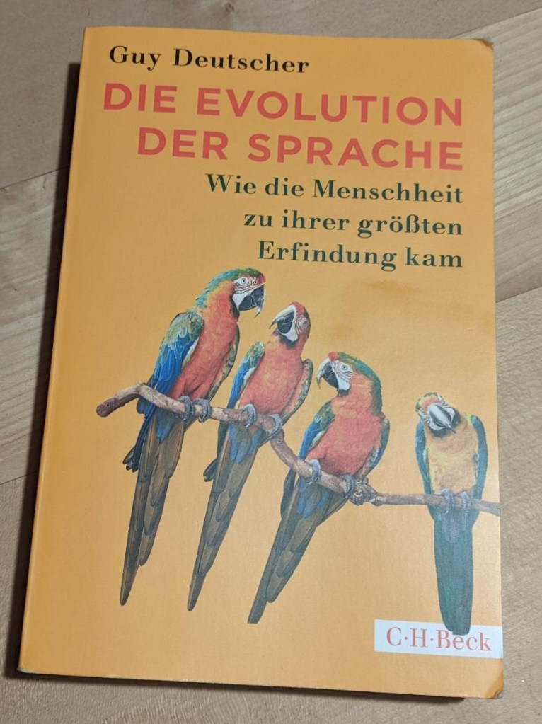
For this year-end write up, I want to discuss the book “The unfolding of language” by Guy Deutscher, which I read this Summer. The book is primarily about linguistics and the evolution of languages, but at the end of this blog post, I will connect some of its ideas with current lines of research in systems neuroscience.
Languages as a pathway to understand thinking
After high school, my main interest was to understand how thoughts work. Among the various approaches to this broad question, I felt that I needed to choose between at least two paths. First, to study the physiology of neuronal systems, in order to understand how neurons connect, how they form memories, concepts, ideas, and finally thoughts. Second, to study the matrix that shapes our thoughts and that itself is formed by the dynamics and connections in our brain: language. I decided for the first trajectory, but I always remained curious about how to use language to understand our brain.
I like languages, especially from the theoretical perspective. I was a big fan of Latin in high school and particularly enjoyed to dive into the structure of its language, that is, its grammar. My mother tongue, German, also offered a lot of interesting and complex grammar to explore. And when I read through the books of J.R.R. Tolkien on Middle-earth, I was fascinated by all the world-building but in particular by the languages that he had invented. And I filled a few notebooks with some (less-refined) attempts to create my own languages. Apart from the beautiful words and the intriguing sounds, I was especially into the structure and grammar of these languages. – Later, I became relatively proficient in a few computer languages like C, Python, LaTeX, HTML or Matlab. I briefly tried to learn Chinese for a year, but although I was fascinated by the logical grammatical edifice, I did not have the same energy to internalize the look-up-tables of characters and sounds. Occupied with neuroscience and mostly reading and writing scientific English (a poor rip-off of proper English), I lost touch with the idea of using language to understand our thoughts and, therefore, the brain.
“The unfolding of language”
Then, Mid of last year, I came across the book The unfolding of language in a small but excellent bookstore at Zurich main station. I was captivated immediately. And I enjoyed the book for several reasons.
First, the book is abundant with examples how language evolves, about the origin of words or grammatical structures. Many details that I never had bothered to consider, made suddenly sense, like some old German words, the French conjugation of verbs, or a certain declination of a Latin word. In addition, I learned a few surprising new principles about other languages, for example, the structure underlying the semitic languages, for which the author is an expert.
Second, the depiction of the evolution of language revealed a systematic aspect to these changes, even across languages even from different language families. I did have some basic knowledge about the language sound changes that had been observed around 1800 and described by Grimm’s law. However, Guy Deutscher’s book did not describe these systematic changes as artifacts of our history but as a natural process that occurred like this or similarly in many different languages, independently from each other. To some extent, reading about all these systematic and – to some extent – inevitable changes of language made me more relaxed about the distortions that language undergoes when used by younger generations or people who mix in loanwords from other languages without hesitation; language is a non-static, evolving object. But what is the evolution of language described by Guy Deutscher actually?
The three principles of the evolution of language
Deutscher mentions three main principles underlying the evolution of language. The strong impression that this book left on me was not only through these principles of language evolution, but even more so through the wealth of examples across languages, types of words and grammars that it provided.
First principle: Economy
“Economy”, according to Deutscher, mostly originates from the laziness of the language users, resulting in the omission or merging of words. One of the examples given in the book was the slow erosion of the name of the month “august” from the Latin word augustus over the Old French word aost to août (which is pronounced as /ut/) in modern French. Such erosion of language appeared as the most striking feature of the evolution of language when it was discovered two centuries ago. It was an intriguing observation that the grammar of old languages like Latin or Sanskrit seemed to be so much more complex than the grammar of newer languages like German, Spanish or English. This observation led to the idea that language is not actually simply evolving but rather decaying.
Deutscher, however, describes how this apparent decay can also be the source and driving force for the creation of new structures. One particular compelling example is his description of how the French conjugation for the future tense has evolved. It is difficult to convey this complicated idea in brief terms, but it evolves around the idea that a late Latin expression like amare habeo (“I have to love”) evolved its meaning (to “I will love”), which was transferred to French, where the futur tense therefore contains the conjugation of the present tense of the word “to have”:
| j’aimerai | i will love | j’ai | i have |
| tu aimeras | you will love | tu as | you have |
| il aimera | he will love | il a | he has |
| nous aimerons | we will love | nous avons | we have |
| vous aimerez | you will love | vous avez | you have |
| ils aimeront | they will love | ils ont | they have |
I knew both Latin and French quite well, but this connection struck me as both surprising and compelling. Deutscher also comes up with other examples of how grammar was generated by erosion, but you will have to read the book to make up your own mind.
Second principle: Expressiveness
Expressiveness comes from the desire of language users to highlight and stress what they want to say, in order to overcome the natural inflation of meaning through usage. A typical example are the simple words “yes” and “no”, which are simple and short and therefore often enhanced for emphasis (“yes, of course!” or “not at all!”).
A funny example given by Deutscher is the French word aujourd’hui, which means “today” and is one of the first words that an early beginner learns about French. Deutscher points out that this word was derived from the Latin expression hoc die (“on this day”), which eroded to the Old French word hui (“today”). To more strongly emphasize the word, people started to say au jour d’hui, which basically means “on the day of this day”. Later, au jour d’hui was eroded to aujourd’hui. Nowadays, French speakers start using au jour d’aujourd’hui to put more emphasis on the expression. Therefore, the expression means “today” but literally can be decoded as “on the day of the day of this day”. This example illustrates the close interaction of the expressiveness principle and the erosion principle. And it shows that we are carrying these multiple layers of eroded expressiveness with our us, often without noticing ourselves.
Third principle: Analogy
“Analogy” occurs when humans observe irregularities of language and try to impose rules in order to get rid of exceptions that do not really fit in. For example, children might say “the ship sinked” instead of “the ship sank”. Through erosion, language can take a shape that does not make any sense (because its history of evolution, which would shine a light on the shape, is not obvious), and we try to counteract and impose some structure.
Metaphors are the connection between the physical world and abstraction
But there is one more ingredient that, according to Deutscher, drives the evolution of language. It is this aspect which I found most interesting and most closely connected to neuroscience: metaphors. This idea might sound surprising at first, but once it unfolds by means of examples, it becomes more and more convincing. Deutscher depicts metaphors as a way – actually, the way – how the meaning of words can become more abstract over time.
He gives examples of daily used language and then dissects the used words as having roots in the concrete world. These roots had been lost by usage but can still be seen through the layers of erosion and inflation of meaning. For instance, “abstraction” as a word comes from the Latin words ab and strahere, which basically means “to pull something off of sth.”, that is, to remove a word from its concrete meaning. “Pulling sth off”, on the other hand, is something very concrete, rooted in the physical word.
Such abstraction of meanings is most obvious for loanwords from other languages (here, from Latin). But Deutscher brings up convincing examples of how this process occurs as well for words that evolved within a given language. To give a very simple example that also highlights what Deutscher means when he speaks of metaphors: in the expressions “harsh measures”, the “harsh” has roots in the physical world, describing for example the roughness of a surface (“rough” or, originally, “hairy”). Later, however, “harsh” has been applied to abstract concepts such as “measures”– originally as a metaphor that we, however, do no longer perceive as such. Deutscher recounts many more examples, which, in their simplicity, are sometimes quite eye-opening. He makes the fascinating point that all abstracts words are rooted in the physical world and are therefore mostly dead metaphors. And how could one not agree with this hypothesis? Because, what else can be the origin of a word if not physical reality?
How metaphors create the grammar of languages
Deutscher, however, even goes beyond this idea and posits that abstraction and metaphors may have created also more complex aspects of language. For example, in most languages, there are three perspectives: me, you and they. He makes the point that these perspectives might have derived from demonstratives. “Here” transforms to “me”, “there” to “you”, and a third word for something more distant “over there” to “they”. All of these words are “pointing” words, probably deriving from and originally accompanying pointing gestures. In English, the third kind of word does not really exist as clearly, but for example Japanese features the threefold distinction between koko (“here”), soko (“there”) and asoko (“over there”). The third category is represented in Latin by the word ille, which refers to somebody who is more distant. As a nice connection, the Latin word ille was the origin for the French word il/ils, which means “he/they”. This shows how the metaphorical use of words related to the physical world (point words) can generate abstract concepts like grammar, here: the third person. Deutscher alos brings up languages where the connection between the three demonstratives for persons of variable distances and the pronouns for me/you/they is more directly visible, for example in Vietnamese.
Therefore, Deutscher plausibly demonstrates how not only abstract words, but also more complex structures that underlie the most basic grammar, are evolved from metaphorical usage of concrete words that are related to the physical world, either because they describe physical things (the surface roughness) or because they are originally only enhancements of gestures (pointing words). These ideas in the book are amongst the most interesting ones that I have encountered for quite some time.
Embedding of “The unfolding of language” in current research
Overall, I like the hypotheses presented by Deutscher. The only issue I have is that there are many missing bits and pieces that prevent me from properly see through all potential weaknesses. I simply don’t know whether these questions are unanswered in general or whether Deutscher did not have enough space to treat them in this (popular science) book. Put differently, the book was very engaging and a fascinating read but did not provide useful links to the research literature. How are all these ideas embedded in current linguistics research, or is all of this Deutscher’s own concepts? I observed that there are some links in this work to ideas like the conceptual metaphor or linguistic relativity, but I was unable to really figure out where to get started if I wanted to dig deeper into the principal role of metaphorical use for the development of grammar and abstraction. If a linguistics expert somehow happens to read this blog post, I’d be really happy to get a recommendation on a standard textbook (if there is any) on these topics and how Guy Deutscher’s work fits in.
Metaphors, abstraction and system neuroscience
However, I’d like to briefly discuss an aspect of the metaphor principle that I found particularly interesting, also because of a potential, albeit loose, link to current research in neuroscience. Many neuroscientists are probably aware of the large branch of neuroscience dedicated to understanding the generation and representation of abstract knowledge. This can take very different forms, but one of the most prominent takes is the idea that the hippocampus and the entorhinal cortex, originally shown to represent space (via the famous place cells and grid cells, respectively), also represents more abstract knowledge.
The entorhinal cortex represents physical space using the above-mentioned grid cells that span space with hexagonal lattices of varying spatial scales. Building upon the hexagonal lattice idea, researchers attempted to apply the concept experimentally to more abstract 2D spaces. For example, such an abstract conceptual space would not be spanned by the physical axes “x” and “y” but for example by the conceptual axes “neck length” and “leg length” of a bird. I have to admit that I was not fully convinced by this approach, but it is interesting nevertheless.
Apart from these experimental approaches, researchers have developed theories about the representation of abstract knowledge based on hexagonal lattices (for an example theory, see Hawkins et al., 2019 or Whittington et al., 2020). Or check out this review of experimental literature that concludes that grid cells reflect the topological relationship of objects, with this relationship being defined either via space or via more abstract connections. These approaches have in common that abstract concepts are built upon the neuronal scaffold; the neuronal scaffold, in turn, is provided by the representation of physical space.
In Deutscher’s book, I found a description that paralleled the above ideas from systems neuroscience, enough to make it intriguing. First, Deutscher posits that all words that now describe abstract relationships are rooted in meanings that represent physical space. More precisely, words that were originally used to describe physical relationships (e.g., “outside”), were later taken to describe an abstract relationship (“outside of sth”, with the same meaning as “apart from sth”). We even don’t notice the metaphorical usage here because it is so common, even across languages (hormis in French, utenom in Norwegian, ausserdem in German). Deutscher highlights one specific field where the transition of spatial to more abtract descriptors is very apparant. “Before”, “after”, “around”, “at” or “on” are all prepositions that describe physical relationships but that were lateron assigned to temporal relationships as well. It seems quite obvious and not worth any further thought, but is it really?
Deutscher not only suggests that spatial relationships are more basic than temporal relationships, but he strengthens this point by pointing out that words that describe physical relationships derived from something even simpler: the own body. For example, “in front of” derives from the French word front (“forehead”). Deutscher brings up many more examples from diverse languages that reveal how the language that describes abstract relationships can be traced back to body parts. Therefore, he hypothesizes that body parts (“forehead”, “back”, “feet”, etc.) were originally used to establish a system of spatial relationships, which was then applied to temporal and other more abstract relationships. It would be interesting to investigate these lines of thought for systems neuroscience (for example, egocentric vs. allocentric coding of position, or how temporal sequences are required to define abstract knowledge representations).
One of the open questions here is about a potential interaction between abstractions, language and neuronal representations. Was this connection already implemented on the neuronal level before the inception of language, such that language only had to use this analogy generator? Researchers who work on abstract knowledge representation in animals like mice would probably say so. Or was it only through language that abstraction was enabled? I find both possibilities equally likely. Often, we cannot use a concept or idea efficiently when we don’t put it into an expression – concepts remain vague and often difficult to judge if we don’t pour them into clear thoughts, ideally written down in a consistent and concise set of sentences.
In the end, I find the ideas about the evolution of language extremely interesting, especially because they relate to the generation of abstract relationships (temporal relationships, language grammar, or fully abstract concepts). From my point of view, two aspects could be worth some further research. First, to dig into the status of the linguistic research on these topics. And second, to understand whether there are any meaningful parallels between abstraction in neuronal representations and abstraction derived within an evolving and eroding language. In any way, I can recommend this book fully to anybody who is not afraid of foreign languages and a bit of grammar.
.
P.S. I’ve read the German version of Deutscher’s book. It is not simply a translation of the English version but provides many additional examples from the German language that enhance or replace the examples taken from English. This was done in an excellent manner, and I can only recommend to German-speaking readers of this blog to read the translation and not the original version.


