Our paper on A database and deep learning toolbox for noise-optimized, generalized spike inference from calcium imaging is out now in Nature Neuroscience. It consists of a large and diverse ground truth database with simultaneous calcium imaging and juxtacellular recordings across almost 300 neurons. We used the database to train a supervised algorithm (“Cascade”) to infer spike rates from calcium imaging data.

If you are into calcium imaging, here are 5 reasons why you should use Cascade.

1. You don’t have to install it

You are not familiar with Python? Or you don’t want to install dependencies? No problem. Click this link. The link will bring you to an online interface where you can work with Cascade. You can upload your data (dF/F traces) as *.mat- or *.npy-files and download the results (inferred spike rates). Trying out the package is as quick as it can get. The online interface is a Google Colaboratory and therefore runs on servers provided by Google for free.

However, you can also install Cascade locally on your computer. Just go to the Github page and follow the installation instructions (tested on Ubuntu, Windows and Mac). This might be useful if you want to integrate spike inference into an existing workflow. People including myself have used Cascade together with CaImAn or Suite2p. You can use the dF/F output of these packages and apply the Cascade “predict” function as seen in the demo scripts. It’s a single-line addition of code to your pipeline.

Personally, I used Cascade with a GPU for the analyses in the paper. For daily work with calcium imaging recordings in mice (typically a few hours of recordings and a few hundreds of neurons), I run it on a computer without dedicated GPU because it’s fast enough on any reasonable CPU (seconds to minutes). Sometimes, I also use the online Colaboratory Notebook. The results are identical, whether I use a local installation or the Notebook, since the code is identical.

2. You don’t have to tune parameters

For each neuron from a data set, the algorithm automatically detects the noise level and chooses an appropriately trained model. The models are trained across many different conditions and indicators. This broadly trained model ideally generalizes to unseen data. Check out Figure 3 in the paper if you want to know more about the details.

To get started, you have to choose a model based on the frame rate of your recordings and on the temporal resolution that you want to achieve with spike inference. The FAQ, which can be found both on the Github Readme and at the end of the Colab Notebook, give you guidance if any doubts remain.

3. Estimate absolute spike rates

Have you ever wondered whether a specific calcium transient corresponded to a single action potential or a burst of many action potentials? At least it would be nice to have some estimate of spike rates for a given recording. Cascade gives you this estimate.

The next question is a bit more tricky: how precise is that estimate? – It is as exact as it can get if you apply an algorithm to calcium imaging data where you do not have an associated ground truth. We have quantified this precision in the paper in terms of correlation (=variance explained), absolute errors and typical biases (see Figure 3 and Extended Data Figure 4). In the end, the typical errors depend on the data quality and noise levels. However, you should expect that the true spike rate might be as low as 0.5 times or as high as 2.0 times the spike rate estimated by Cascade. On average across neurons, the error will be lower. This is not single-spike precision, but, as bad as it sounds, this is as good as it gets. The imprecision is, among other things, due to the unpredictable heterogeneity of the spike-calcium-relationship across neurons.

However, absolute estimates with a certain imprecision, which you get from Cascade, are still better than results that do not have an immediate meaning (dF/F scores).

4. Improve temporal precision

Spike inference, also referred to as temporal “deconvolution” of calcium recordings, improves the temporal resolution by getting rid of the slow calcium transient. The slower the calcium transient, the more pronounced the improvement of deconvolution. And, yes, the algorithm generalizes well across short and long time constants.

Applications where I have used Cascade myself to achieve improved temporal resolution:

a) Detection of fast sequences on a sub-second time scale (check out Figure 5e in our toolbox paper)

b) Detection of swimming-locked neuronal activity in head-fixed adult zebrafish. Adult zebrafish move on a sub-second time scale, faster than the calcium indicators we used in their brains at room temperature.

c) Locking of neuronal activity to oscillations in the hippocampus (ongoing work, not yet published).

If your observations are masked by slow indicator transients, give it a shot and try out Cascade.

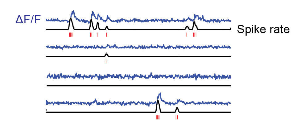
5. De-noise your recordings

When I used Cascade for the first time, I was surprised how well it de-noised recordings. The Cascade paper is full of examples where this is validated with ground truth.

Or, have a look at the spike rate predictions for the Allen Brain Observatory data set (Figure 6b,f,g,h; Extended Data Figure 10). Shot noise is removed, and slower transients due to movement artifacts are rejected. The algorithm simply has learned very well how an action potential looks like.

One of the most striking examples, however, was when we tested the effect of Cascade on population imaging analyses (Supplementary Figure 11, the only figure not yet included in the preprint). To this end, we used NAOMi to simulate neuronal population patterns and analyzed how well the correlations between neuron pairs were predicted from dF/F traces (red) or from spike rates inferred with Cascade (blue). For dF/F traces, correlations were often overestimated (among other reasons due to slow calcium transients) and underestimated (due to overwhelming noise). Pairwise correlation computed from Cascade’s spike rates are simply closer to the true correlations.

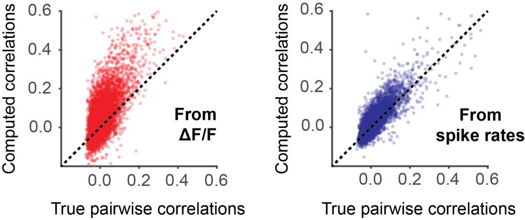
Therefore, if you want to get the best out of your 2P calcium imaging data, I would recommend to use Cascade. The result is simply closer to the true neuronal activity.