On Twitter, Richie Hakim asked whether the toolbox Cascade for spike inference (preprint, Github) induces temporal dispersion of the predicted spiking activity compared to ground truth. This kind of temporal dispersion had been observed in a study from last year (Wei et al., PLoS Comp Biol, 2020; also discussed in a previous blog post), suggesting that analyses based on raw or deconvolved calcium imaging data might falsely suggest continuous sequences of neuronal activations, while the true activity patterns are coming in discrete bouts.

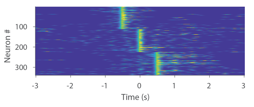
To approach this question, I used one of our 27 ground truth datasets (the one recorded for the original GCaMP6f paper). From all recordings in this data set, I detected events that exceeded a certain ground truth spike rate. Next, I assigned these extracted events in 3 groups and systematically shifted the detected event of groups 1 and 3 by 0.5 seconds forth and back. Note that this is a short shift compared to the timescale investigated by the Wei et al. paper. This is how the ground truth looks like. It is clearly not a continuous sequence of activations:

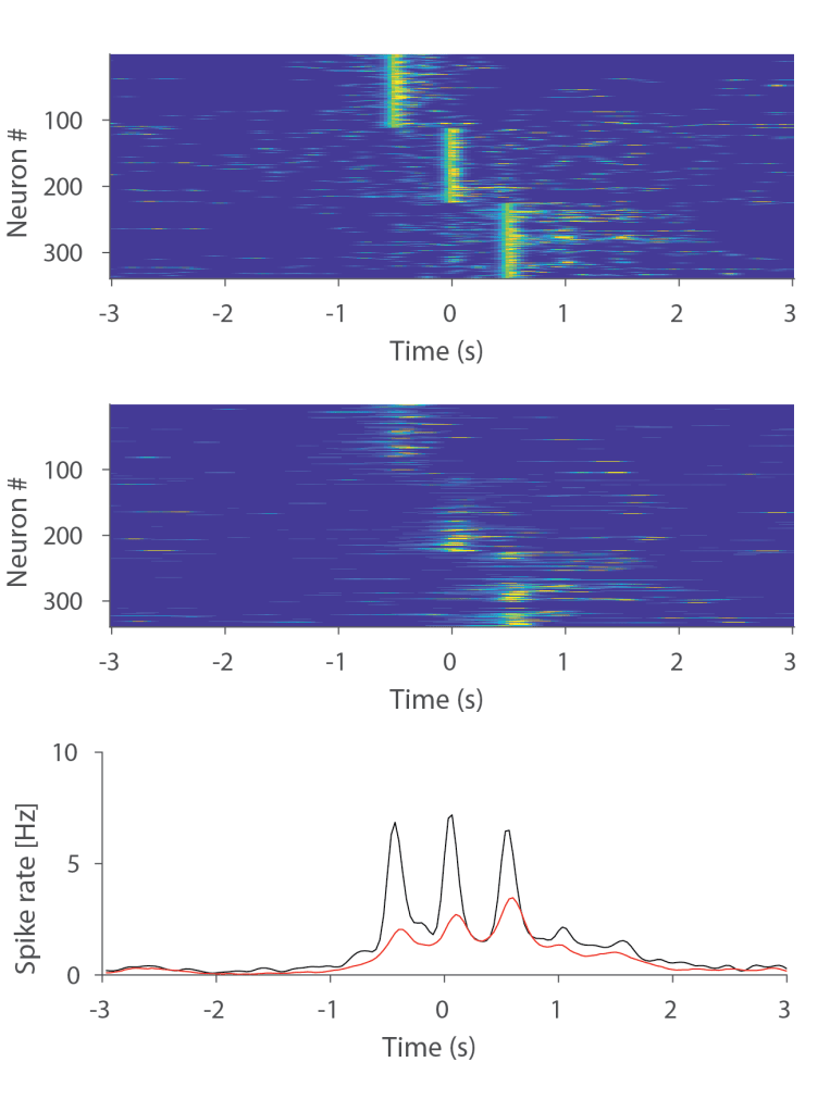
To evaluate whether the three-bout pattern would result in a continuous sequence after spike inference, I just used the dF/F recordings associated with above ground truth recordings and Cascade’s global model for excitatory neurons (a pretrained network that is available with the toolbox), I infered the spike rates. There is indeed some dispersion due to the difficulty to infer spike rates from noisy data. But the three bouts are very clearly visible.

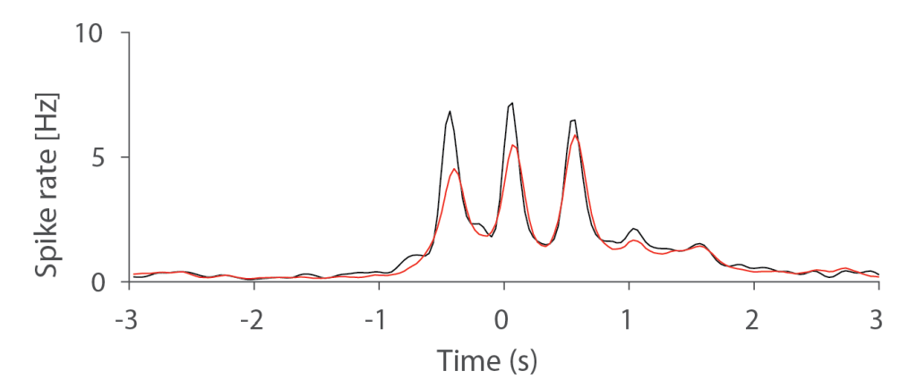
This is even more apparent when plotting the average spike rate across neurons:

Therefore, it can be concluded that there are conditions and existing datasets where discrete activity bouts can be clearly distinguished from sequential activations based on spike rates inferred with Cascade.

This analysis was performed on neurons at a standardized noise level of 2% Hz^-1 (see the preprint for a proper definition of the standardized noise level). This is a typical and very decent noise level for population calcium imaging. However, if we perform the same analysis on the same data set but with a relatively high noise level of 8% Hz^-1, the resulting predictions are indeed much more dispersed, since the dF/F patterns are too noisy to make more precise predictions. The average spike rate still shows three peaks, but they are only riding on top of a more broadly distributed, seemingly persistent increase of the spike rate.

If you want to play around with this analysis with different noise levels or different data sets, you do not need to install anything. You can just, within less than 5 minutes, run this Colaboratory Notebook in your browser and reproduce the above results.