Most neuroscientists who analyze their data themselves use either Matlab or Python or both – the use of R is much less common than in other fields of biology. I’ve been working with Matlab on a daily basis for >10 years, and I have started using Python regularly, although less frequently, about 5 years ago. I’d like to encourage everybody to learn Python, because the language is much more flexible, more beautiful and more powerful. But still I use Matlab often to get a first impression of data, because it is simply perfect for browsing intermediately sized (MB to GB) datasets and for doing simple things in general, also due to the plotting interfaces which I find are easier to use for data exploration than matplotlib/seaborn in Python.

Here, I would like to share a collection of useful Matlab commands which are not complicated or fancy but still nice to know. Don’t expect too much, and don’t read this if you have spent a couple of years with Matlab already. To be entirely honest, I’m writing this also for my own reference, because I keep forgetting the exact wording of some of the commands, and it’s nice to have everything in a single place. Without further ado, here is my list of favorite Matlab spells:

1. Leading zeros with sprintf()
2. Automatization with dir()
3. Exclude file patterns based on regular expressions
4. Callback functions to speed up image inspection
5. Regionprops for image segmentation
6. The curve fitting toolbox
7. Manually modifying colormap
8. Turning the background of a figure white
9. Make ticks point outwards instead of inwards
10. Rotate x-tick labels
11. Reverse y-axis direction
12. Save large figures to vectorized format (eps)
13. Get raw data from figures
14. Position the figure window at a given screen location
15. Profiling code with tic/toc

1. Leading zeros with sprintf()

Imagine you’re going through a for-loop and want to save a file for each loop iteration, with a filename that contains the loop index. This can become a real mess and often ends up in a list of files that is difficult to sort, e.g.:

‘Dataset2_trial1.mat’
‘Dataset2_trial12.mat’
‘Dataset2_trial13.mat’
‘Dataset2_trial2.mat’
…

To circumvent this problem, you can include leading zeros. This is how it is done:

for index = 1:13
   index_with_zeros = sprintf('%03d',index);
   filename = ['Dataset2_trial',index_with_zeros,'.mat'] ;
   rand_matrix = rand(256);
   save(filename,'rand_matrix')
end

Resulting in the following output:

‘Dataset2_trial01.mat’
‘Dataset2_trial02.mat’
‘Dataset2_trial03.mat’
‘Dataset2_trial04.mat’
…

Much better!

2. Automatization with dir()

You want to go through a set of folders. Let’s say, all of them contain in their name the string “to_be_analyzed” somewhere in the middle. In each folder, there are files that you want to process, but only those that start with “Neuron7” and end with “.mat”.

That’s how this is done, with the beautiful dir() command:

folder_list = dir('*to_be_analyzed*');
for k = 1:numel(folder_list)
   cd(folder_list(k).name);
   file_list = dir('Neuron7*.mat");
   for j = 1:numel(folder_list)
      load(folder_list(j).name);
      % perform operations on loaded data
    end
    cd ..
end

Very easy, very simple, and saves the cost of going manually through folders and files. Many people are spending days and weeks with renaming and manually loading datasets. This can be done much faster, even in Matlab.

3. Exclude file patterns based on regular expressions

However, sometimes the dir() command is a bit tricky to use. Imagine you have the following files:

‘Dataset2_trial01.mat’
‘Dataset2_trial01_processed.mat’
‘Dataset2_trial02.mat’
‘Dataset2_trial02_processed.mat’
…

How can you get only those files without the ‘_processed’ ? This is, unfortunately, not trivial. However, the following piece of code does the trick:

file_list = dir('Dataset2_trial*.mat');
file_list = file_list(~endsWith({file_list.name},'processed.mat'));

This is using regular expressions, something which Python can do much better. But Matlab also has these functionalities – you just have to know the magic spell!

4. Callback functions to speed up image inspection

Let’s say you want to manually inspect 10’000 images, whether the image is useful or not. How to do this in the most efficient way? The solution to this problem are keyboard callback functions. I have written a blog post before on this topic, including a minimal working example consisting of few lines of code.

I have seen so many times people going through images and writing down an annotation sheet in Excel in parallel. This is highly inefficient, and callback functions attached to figures in Matlab solve this problem with very little code. Going through the 10’000 images will take you 3 hours, instead of 3 days.

5. Regionprops for image segmentation

Imagine you have a binary image and want to measure the number of objects and its properties. Matlab comes with an extremely powerful set of functions for image analysis. The function regionprops() is a good starting point and very user-friendly. You can just insert a couple of arguments and you get not only the number of objects, but also the area, the center of mass, the convex hull, the orientation of the object, and much more. If you want to write a very small and user-friendly tracking software in Matlab, this is the way to start.

6. The curve fitting toolbox

Many people think that fitting in Matlab is difficult. It is not really. The curve fitting toolbox does not come for free, but if you have the choice, do get it!

You can open the curve fitting toolbox using this simple spell:

cftool

This will open the fitting toolbox graphical user interface, which is very intuitive to use in my opinion. For example, you can perform fits on custom-defined functions, and you can change the initial guesses for the fit parameters (which can make a huge difference for the success of your fit!). It’s the perfect way to play around and explore fits of different functions to your data.

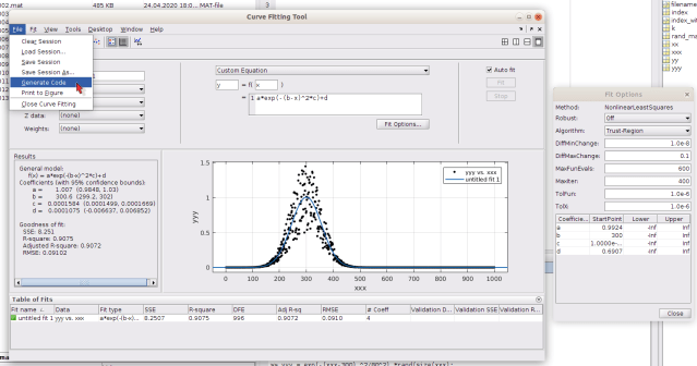
The best feature of this graphical user interface, however, is the “Generate Code” option (highlighted in the screenshot). This allows you to first explore the data manually, and then generate code which performs the same fit. It is much more difficult to find out all those commands and fitting options through web searches. Therefore it is very convenient to use cftool for exploratory fitting and setting up automatized code.

7. Manually modifying colormaps

Let’s say you have a density plot, but you’re unhappy with the colormap. Maybe you are using the “gray” colormap, but you want to have it the other way around, with black for high values and white for low. Or you want to have the top value in a different color (e.g., red, for saturating). For example, instead of using the standard “parula” colormap (left), the inverted colormap (right), with the highest values set to a custom color (white):

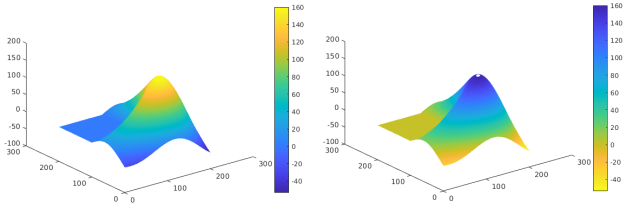
Here is the code to achieve this. The colormap is saved into the variable “cmap”:

% mess around with the colormap
cmap = parula(256);
cmap = cmap(end:-1:1,:);
cmap(end,:) = [1,1,1];

% make a figure that uses this colormap
figure(31);s = surface(L);
s.EdgeColor = 'none';
colormap(cmap)
view(3)

Easy!

8. Turning  the background of a figure white

If you want to export a figure as PNG, or if you simply want to make a screenshot of a plot without an ugly border around it, you can simply set the background to white:

set(gcf,'color','w');

Very simple! By the way, “gcf” means something like “get current figure handle”, so it will apply to the most recently active figure.

9. Make ticks point outwards instead of inwards

Some people have a strong preference whether ticks in scientific plots should point inwards or outwards. Since the Matlab default is “inwards”, here is the magic command to let them point outwards:

set(gca,'TickDir','out');

Related, adjusting the length and thickness of the ticks is sometimes a good idea:

ax = gca;
ax.TickLength =[0.02 0.01];

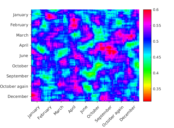
10. Rotate x-tick labels

Sometimes, the x-tick labels are simply too large and don’t have place next to each other. The solution is to rotate them:

figure, imagesc(matrix_smoothed);
xticks([10 20 30 40 50 60 70 80 90])
xticklabels({'January', 'February','March','April','June',...
   'October','September','October again','December'})
xtickangle(45)

For a rotation of x-tick labels by 45°. In earlier versions of Matlab (<Matlab 2016), a slightly more complex command does the same:

set(gca, 'XTickLabelRotation',45)

11. Reverse y-axis direction

Matlab is very particular about the direction of the y-axis in its plots. And it’s also not really consistent between different commands (e.g., plot() vs. imagesc() ). In order to force Matlab to reverse the direction of the y-axis, you can use the following command:

% reverse:
set(gca, 'YDir','reverse')
% back to normal:
set(gca, 'YDir','normal')

There is another command which does the same but is considerably shorter, but also less intuitive:

% reverse:
axis ij
% back to normal:
axis xy

12. Save large figures to vectorized format (eps)

The art of reliably saving figures to beautiful vector graphics has not yet been discovered for Matlab. The first rule I learnt is to avoid anything related to transparency (it can be added later in a vector graphics program more easily).

Personally, I like exporting figures as *.eps-files. However, for files with many datapoints, newer versions of Matlab per default do not save a properly vectorized figure any more. This behavior can be circumvented by manually telling Matlab how to export the eps explicitly. The following piece of code properly exports the current figure to the file “methusalem.eps”:

print -painters -depsc methusalem.eps

13. Get raw data from figures

It does not happen in the ideal world, but sometimes the original data are lost or difficult to generate and there is only a figure saved as “XYZ.fig” in a folder which contains the data as plots. Fortunately, it is very easy to extract the data from plots if you know the key word. Just open the figure in Matlab. Then, it’s a one-liner:

handle = get(gca);

Afterwards, type in “handle” in the console, and you will be able to search for the data. Something like “handle.Children.CData” will be the data for an imagesc() figure and “handle.Children.YData” will be the data for the case of a plot() figure. You will find it out easily.

Alternatively, select the plot of interest with the cursor and get a handle on this object directly:

handle = get(gco);

14. Position the figure window at a given screen location

Making 23 similar plots is no fun if you decide that the plot window should be smaller or larger or positioned in a different screen location. Dragging the window manually simply costs a lot of time. The following command performs this operation automatically:

x_location = 199
y_location = 302
width = 600
height = 300
set(gcf, 'Position', [x_location y_location width height]);

Not many people seem to use these commands on a regular basis, although I find them essential for reproducible figure sizes and for automatization. If you are working with two screens, you might have to play around with negative coordinates as well.

15. Profiling code with tic/toc

There is the proper way to benchmark code and to find out how long each command takes; and then there is tic/toc –  which I actually use very frequently. When the “tic” command is executed, a timer starts counting seconds. “toc” is the variable that points to this timer, and the respective value can be assigned to a variable.

For example, the following code

tic
Random = rand(10000);
toc
Random = Random.^Random;
toc

gives the following result in the command line:

Elapsed time is 0.910930 seconds
Elapsed time is 2.862613 seconds,

indicating that the first command, rand(10000), took 0.9 seconds, while the other one took 2.9 – 0.9 = 2.0 seconds.

I hope you learnt something new today! Or, if not, leave a comment with your favorite simple Matlab spell!