When reading through the first informative web pages on transfer entropy, it turns out how closely its concept is related to mutual information, and even closer to incremental mutual information; and, although it’s based on a totally different approach, it tries to create a measure of time-shifted influences similar to Granger-causality. The main difference: the latter is based on simple linear fit prediction, whereas the former is based on information theory.

I haven’t found something in the net which explains transfer entropy in simple pictures for the layman – quite a shame, considering the attention transfer entropy has recently gained in neuroscience. So I will refer to a highly cited article by Thomas Schreiber, which is freely available in the arXiv (link). On the first two pages, almost everything which is needed is explained. I suppose, however, that Schreiber’s background is theoretical physics.

It’s instructive to compare mutual information with transfer entropy. Mutual information quantifies the reduction in uncertainty about a time series X by knowing about the time series Y (at the same time points), see my previous post. Transfer entropy, on the other hand, quantifies the reduction in uncertainty about a time series X, when both the past of X and the past of Y is known. Mathematically speaking, mutual information is:

This is basically nothing but the probability of x under no special condition – – compared to x under the condition of y: .

Similarly, transfer entropy is the probability of x under the condition of its own past (let’s name it X) – – compared to the probability of x under the condition of the past of both variables: :

The rest is implementation details: determining the time bin size and calculating the transfer entropy out of the data and their probability distributions. I found an easy-to-use Matlab package which can be applied for spiking data, i.e. binary values for the variables, available on GoogleCode (link to code, paper which uses code; the paper itself seems to be less interesting). You have to compile a mex-file to use the code.

Unfortunately, I had no spike data, so I decided to derive artificial spike data from my C. elegans calcium imaging traces. I normalized each trace to the range [0;1]. Then I created a binary time course by attributing ones and zeros with the probability given by the normalized calcium fluorescence intensity. By averaging over 1000 of such binary pseudo-spiking traces, the original normalized traces are recovered. As the transfer matrix method works with distributions, this trick works. Of course, it is not the most proper way for demonstration, but the data are anyhow not the gold-standard for connectivity experiments.

Let’s have a look at the results. Again, we have something similar to the well-known correlation matrix, but it rather is a time lag-dependent transfer matrix. I arbitrarily decided to average over the time lags of 1.5-5 sec. (An average over 0.1-5 sec would have resulted in almost the same matrix. If there existed a non-compressed gif-format, I could have shown the transition.)

Transfer entropy matrix, averaged over delays of 1.5-5 sec.

This looks like a mixture of correlation/mutual information matrizes and Granger causality: let’s look at all of them together.

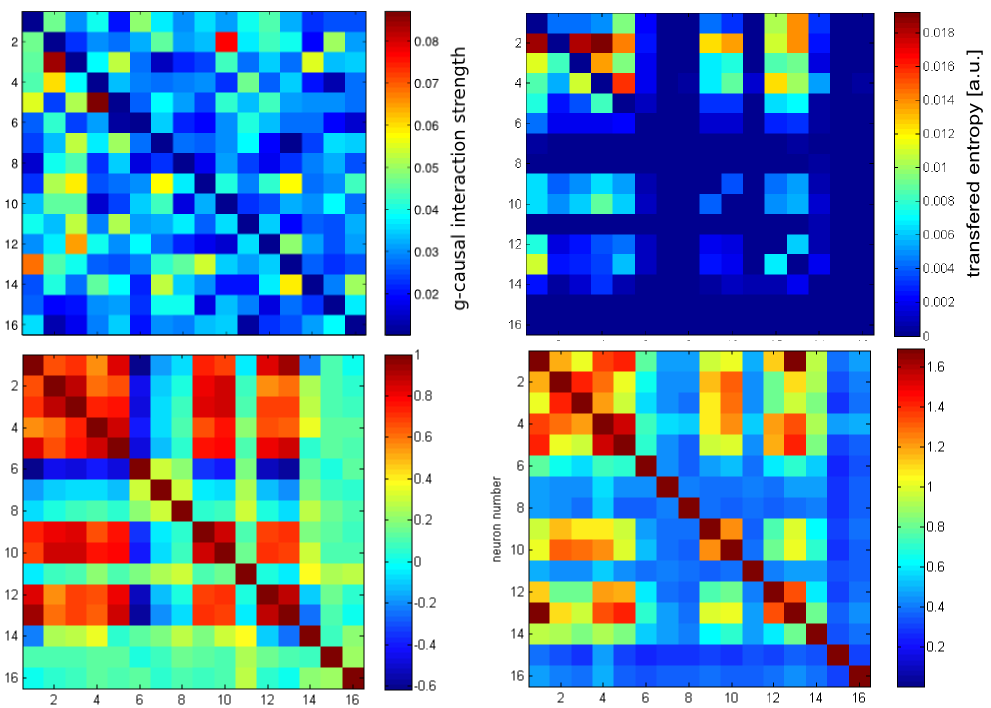
Upper left: Granger causality matrix. Upper right: Transfer entropy matrix. Lower left: Correlation matrix. Lower right: Mutual information matrix. The diagonal elements in the upper row are omitted.

Now I understand why incremental mutual information has been cited (cf. my recent blog post) as an improvement compared with transfer entropy: At least in my data, transfer entropy seems to be no purely causal measure, but is contaminated by correlations; maybe due to similar inputs for some neurons.

Additionally, it is clearly visible that if the data do not yet show a clear causal relation (or are even generated using a simulated deterministic network), it is hard to discriminate causality from correlation and from noise. For scientific analysis, in my opinion, 1) deeper understanding of the data, of the binning, and of the algorithm is required, 2) better data is helpful and 3) a good intuition is essential of what really happens in the network and at which connections it is worth looking more precisely.