Granger causality has been named after the econometrician Clive Granger and has been adapted in the last 10-15 years as time-series analysis tool for neuroscience. The best account for this topic that I have found, is on scholarpedia again (link). The idea is quite simple: you have a timeseries (e.g. activity trace) X, and a timeseries Y. You want to know if the past of timeseries Y can, in addition to the past of timeseries X itself, help to predict the future of timeseries X. Prediction here is nothing but linear regression, somehow a mixture of auto- and cross-regression (copied from scholarpedia):

As it is a linear system, the coefficients of the linear predictor can be calculated easily by using Matlab linear algebra. For clarity, I changed the variables, but this is how it looks like in the Matlab code (lines 71ff. of cca_granger_regress.m):

% solving the linear equation system
Aij = timeshiftedX\X;
% using the solution to predict the future
X_prediction = timeshiftedX*Aij;
% compare data and prediction, leading to regression error
difference = X-X_prediction;

If the regression ‘error’ is reduced by the taking into account the cross-regression part (i.e., in order to predict the future of X, to use not only the past of X, but also the past of Y) significantly, then Y is defined to ‘Granger-cause’ X. ‘Significantly’ of course means that (intransparent) statistical tests are involved. The tests tell you if a connection is g-causal or not, finally leading to a binary result (causal connectivity matrix). This is most likely due to historical reasons. In econometrics, a time series is causal to another one or not. The main author of the scholarpedia article, Anil Seth, also provides a GNU-licenced Matlab package (link to homepage [Update 06-2015: new, modified version, which I tested under Linux]) which turns out to be working nicely out of the box (Matlab 2009b, Windows 7). I couldn’t compile the mex-file, but this file is not necessary for basic testing. [Update: problem solved, took me 4 hours :/] The package is very well documented and easy to understand; it is furthermore accompanied by a very instructive demo. – I applied the basic functions on my dummy C. elegans data in order to be able to compare the methods more easily.

Interaction matrix computed with Granger causality.

When I compare this to the correlation / mutual information matrices in earlier posts, the connections between the neurons seem to be quite sparser. This is simply due to the fact that g-causality looks at (g-)causality, and not correlation; if two timeseries X and Y are identical, then the correlation is maximal; whereas the predictive value of timeseries X for timeseries Y in addition to timeseries Y itself is zero. The redundancy and global behaviour in my C. elegans data evidently shows high correlation, but only little g-causality (as far as these data allow for a statement like this). When I have a look at these g-causal links from neuron 2 to neuron 3 and from neuron 4 to neuron 5, I don’t really see this causality in the temporal traces. But well, this may also be due to my data. The figure should be good enough to give an idea, however. Based on values for statistical significance, a binary connectome can be plotted with the Matlab package:

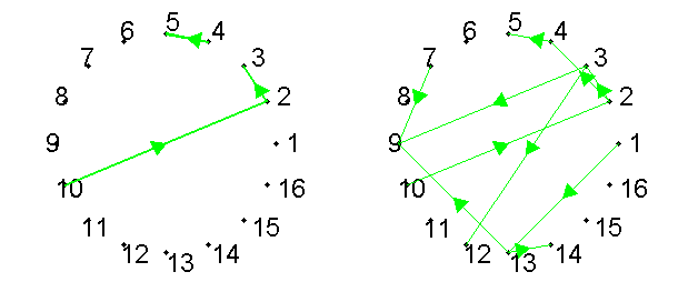
Connectivity diagram, with the numbers indication the neurons. Left: Highly significant connections. Right: Lower significance level.

To sum it up, G-causality is an interesting method which I would like to re-visit later. The outcome is not an improvement of the correlation matrix, but something different. The Matlab package by Anil Seth is easy to understand and useful. As a drawback, the method of linear regression is intransparent, because you only find out if e.g. timeseries Y can help to predict timeseries X, but there’s is no measure about the nature of this influence. When you look into the details, there is a lot of stuff which must be improved, but most of this is already covered e.g. by this Matlab package. In order to be able to apply it succesfully to a data set, one has to dive deeper into things than I have done today.