Last time, I mentioned a website which gives an overview of methods to analyze neuronal (and other) networks. Let’s have a closer look. Here’s a list of the methods:

• Cross-correlation (the standard method)
• Mutual Information
• Incremental Mutual Information
• Granger Causality
• Transfer Entropy
• Incremental Transfer Entropy
• Generalized Transfer Entropy
• Bayesian Inference
• Anatomical Reconstruction

To be honest, I never heard of most of them. So let’s simply go into it and start with ‘Mutual Information’.

It is based on entropy reduction. Entropy is a measure for the uncertainty about a variable. So, mutual information is the reduction of uncertainty about a variable X if you know everything about another variable Y. Here is the definition (Peter E. Latham and Yasser Roudi (2009) Mutual information. Scholarpedia, 4(1):1658):

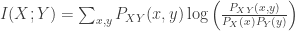
These probability distributions can be thought of as the distribution of the membrane voltage or activity values of single neurons or bigger brain areas. If two activities are completely correlated, the one activity contains all information about the other neuron, i.e., the mutual information is high; if they have nothing to do with each other – in other words: , which eliminates the logarithm -, the mutual information is zero.

So what is the difference to cross-correlation, except for the fact that the formalism seems to be more complicated? Imagine a szenario where the activity of neuron X is not correlated to the activity of neuron Y, but to the square or cube of the activity of neuron Y. This is something which would not be captured appropriately by a simple correlation analysis which is based on covariance ; but it would be captured e.g. by the measure or – and also by mutual information. Is this likely to play a role? Maybe yes. Information processing in neurons is highly non-linear (there is a threshold and a saturation for firing activity, and only a small regime of the input/output-curve can be linearized).

Our point of departure mentions that this method is not appropriate for calcium imaging data. I do not really see this point. So let’s simply try out this formalism on the data which I analyzed in the last post.

To get a distribution from the data, we can either fit a smooth distribution, or we can use bins (say, 15-30 bins for every neuron) and thereby create a discrete probability distribution function (like, a histogram). If we create too many bins, we would not find any mutual information; if we create only two bins for each neuron (corresponding to on/off), we would certainly detect some mutual information. Also, you could imagine taking non-equidistant activity bins.

Some very ugly nested for-loops in Matlab later (number neurons x number neurons x number bins x number bins), I get . It is instructive to draw it like the correlation matrizes:

Left: Correlation analysis matrix. Right: Mutual information analysis matrix. Note that the values on the the diagonal are higher and not all the same for the mutual information matrix.

Looks quite – similar … but there are some differences:

1. Anticorrelation (Neuron #6) is not shown with a specially low value; this is to be expected, as information “doesn’t care about the sign”, contrary to correlation analysis. From correlation analysis, it looks like really strong correlation, whereas mutual information shows that the information dependence of these neurons is not as high for the anti-correlated as for the correlated neurons. Whom should we trust? Nobody of course.
2. The diagonal elements don’t have all the same value (for correlation matrizes, it is always 1). I don’t know if this is important or not.
3. Neuron #4 shows a strange information dependence on the noise neurons #7-8,9,15-16. This is an artefact. It also remains if I shuffle the activity of all neurons temporally, so that every correlation should be destroyed. Where does this artifact come from? – When I created the probability distributions, I divided the activity for each neuron in 25 bins. For most neurons, this gave roughly a gaussian profile. For neuron #4, however, it’s rather like silence most of the time, whereas the activity is limited to small time windows (cf. last blog entry, fig.1). Therefore, by this procedure, most of the time points fall into the first, ‘low activity’ bin. This leads to a high value in the denominator of the formula for this bin, which leads to a very low value for the argument of the logarithm, which leads to a very high value for the logarithm; which in turn is sufficient to pretend information exchange. From which follows, you need to write more sophisticated algorithms in order to overcome such problems.