There are many papers out that use calcium imaging of a lot (tens to thousands) of neurons in animal brains. When I first encountered these kind of publications (roughly a year ago), it took me some hours to become familiar with the mode of presentation, which was very often a correlation matrix.

Yesterday, I was testing my 2-photon widefield microscope on C. elegans with nuclear GCamp5-labeled neurons. So I had the opportunity to do this kind of analysis on my own. Note that 1) I don’t know very much about these neurons 2) I don’t care really much; I’m more interested in the ways of analyzing this kind of data. Here is the neuronal activity of 16 neurons; I labeled them manually in ImageJ:

Neuronal activity of 16 cells in the brain (around the pharynx) of C. elegans.

What’s next? Let’s see how the activity of the neurons are correlated. For this, I simply use the Matlab command corr().

Correlation analysis of the neuronal activity traces.

The correlation matrix makes clear what is already quite evident from the neuronal traces: A bunch of neurons seems to be quite synchronized, namely the neurons 1-5,9-10,12-13. The rest of the neurons seem to be highly anti-correlated (neuron number 6) or rather indifferent (maybe their signal is also too noisy).

But I always was intrigued by the fact that this correlation analysis throws away most of the temporal information, simply by a) taking an instantaneous measurement and b) by averaging over the whole time series. During my diploma thesis, I had to do with particle image velocimetry (PIV) and dual focus correlation spectroscopy (similar to FCS), both of which involve pair/cross correlation functions (note the difference between correlation and the time-dependent correlation function). Autocorrelation functions are a nice way to find temporal patterns, and crosscorrelation is a nice way to find spatio-temporal patterns, i.e., how does neuron A at time t1 influence neuron B at time t2. Let’s try this out for neuron number #1, using the Matlab command xcorr():

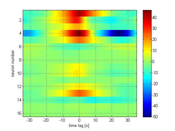
Correlation of neuron #1 with itself (trace 1) and the other 15 neurons.

Let’s just look on time lags less than 30 sec, assuming that events longer away won’t influence the neuron in the presence. We see (in the first row) the autocorrelation function, from which we learn that the average time which passes until the neuronal acitivity changes significantly, is ~10 sec for neuron #1.

From the cross-correlation function in row #2, we see that the activity of neuron #2 seems to advance the activity of neuron #1, and finishes earlier. More general, in most of the neurons which seemed to be simply synchronized according to the correlation analysis, the cross-correlation analysis reveals a temporal, maybe even sequential order of activity.

Of course, this recording of spontaneous acitivity is too short to allow to infer about the directional connectivity. And C. elegans has non-spiking neuronal activity, which makes it less interesting for correlation function analysis.

But this would be the idea. Some weeks ago, I was made aware of the fact that in computational neuroscience or even more theoretical branches of physics/mathematics, there are a bunch of methods which is designed for exactly this task: Here is an overview of methods which might be useful for this task. Probably, not all of these methods will be useful. But maybe some will.