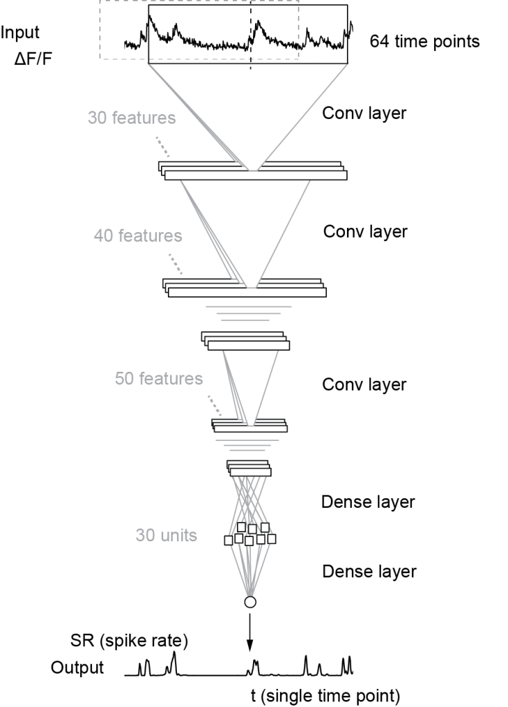
To infer spike rates from calcium imaging data for a time point t, knowledge about the calcium signal both before and after time t is required. Our algorithm Cascade (Github) uses by default a window that is symmetric in time and feeds this window into a small deep network to use the data points in the window for spike inference (schematic below taken from Fig. 2A of the preprint; CC-BY-NC 4.0):

However, if one wants to perform spike inference not as a post-processing step but rather during the experiment (“online spike inference”), it would be ideal to perform spike inference with a delay as short as possible. This would allow for example to use the result of spike inference for a closed-loop interaction with the animal.

Dario Ringach recently came up with this interesting problem. With the Cascade algorithm already set up, I was curious to check very specifically: How many time points (i.e., imaging frames) are required after time point t to perform reliable spike inference?

Using GCaMP/mouse datasets from the large ground truth database (the database is again described in the preprint), I addressed this question directly by training separate models. For each model, the time window was shifted such that a variable number of data points (between minimally 1 and maximally 32) were used for spike inference. Everything was evaluated at a typical frame rate of 30 Hz, and also at different noise levels of the recordings (color-coded below); a noise level of “2” is pretty decent, while a noise level of “8” is quite noisy – explained with examples (Fig. S3) and equations (Methods) again in the preprint.

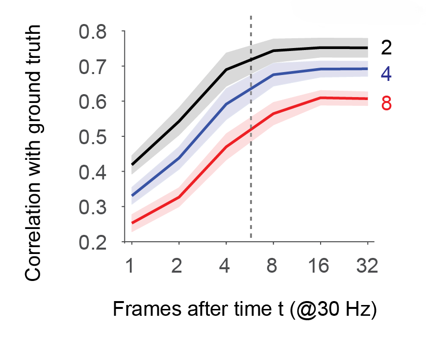
The results are quite clear: For low noise levels (black curve, SEM across datasets as corridor), spike inference seems to reach a saturating performance (correlation with ground truth spike rates) around a value of almost 8 frames. This would result in a delay of almost 8*33 ms ≈ 260 ms after a spiking event (dashed line).

But let’s have a closer look. The above curve was averaged across 8 datasets, mixing different indicators (GCaMP6f and GCaMP6s) and induction methods (transgenic mouse lines and AAV-based induction). Below, I looked into the curve for each single dataset (for the noise level of 2).

It is immediately clear that for some datasets fewer frames after t are sufficient for almost optimal spike inference, for others not.

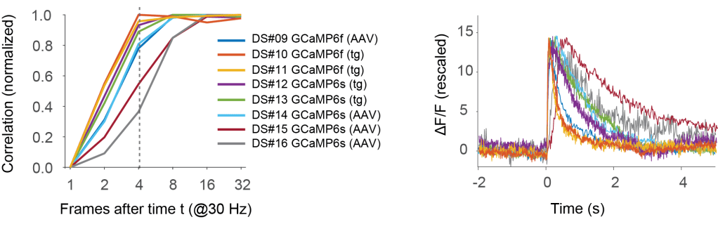
For the best datasets, optimal performance is already reached with 4 frames (left panel; delay of ca. 120 ms). These are datasets #10 and #11, which use the fast indicator GCaMP6f, which in addition is here transgenically expressed. The corresponding spike-triggered linear kernels (right side; copied from Fig. S1 of the preprint) are indeed faster than for other datasets.

Two datasets with GCaMP6s (datasets #15 and #16) stand out as non-ideal, requiring almost 16 frames after t before optimal performance is reached. Probably, expression levels in these experiment using AAV-based approaches were very high, resulting in calcium buffering and therefore slower transients. The corresponding spike-triggered linear kernels are indeed much slower than for the other GCaMP6s- or GCaMP6f-based datasets.

The script used to perform the above evaluations can be found on Cascade’s Github repository. Since each data point requires retraining the model from scratch, it cannot be run on a CPU in reasonable time. On a RTX 2080 Ti, the script took 2-3 days to complete.

Conclusions:

1. Only few frames (down to 4 frames) after time t are sufficient to perform almost ideal spike inference. This is probably a consequence of the fact that the sharp step increase is more informative than the slow decay of a spike-triggered event.
   
2. To optimize the experiment for online spike-inference, it is helpful to use a fast indicator (e.g., GCaMP6f). It also seems that transgenic expression might be an advantage, since indicator expression and calcium buffering is typically lower for transgenic expression than for viral induction, preventing a slow-down of the indicator by overexpression.