Custom-built microscopes have become more and more sophisticated over the last years to provide a larger FOV, better resolution through some flavor of adaptive optics or simply more neurons simultaneously. Professional optical engineers are hired to design the ideal lens combination or the objectives with Zemax, a software that can simulate the propagation of light through lenses systems based on wave optics.

Unfortunately, these complex design optimizations might discourage users from trying to understand their microscopes themselves. In this blog post, I will give a few examples how optical paths of microscopes can be understood and, to some extent, also designed using simple geometrical optics. Geometrical optics, or ray optics, are accessible to anybody who is willing to understand a small equation or two.

Three examples: (1) How to compute the beam size at the back focal plane of the objective. (2) How to compute the field of view size of a point scanning microscope. (3) How to compute the axial focus shift using a remotely positioned tunable lens.

All examples are based on a typical point scanning microscope as used for two-photon microscopy.

(1) How to compute the beam size at the back focal plane of the objective

The beam size at the back focal plane is the limiting factor for the resolution. The resolution is determined by the numerical aperture (NA) focusing onto the sample, and a smaller beam diameter at the “back side” of the objective can result in an effectively lower NA compared to what is possible with the same objective and larger beam diameter.

In general, it is therefore the goal to overfill the back focal aperture with the beam (check out this review if you want to know more). However, especially for video-rate two-photon microscopy, one of the scan mirrors is a resonant scanner, which usually comes with a usable aperture of ca. 5 mm. Often, there are only two lenses between scan mirror and objective, scan lens and tube lens. The two black lines illustrate the “boundaries” of the beam:

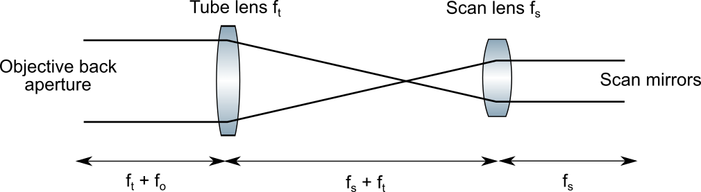
If the beam diameter at the scan mirror is 5 mm, the beam diameter d_BFA at the objective’s back aperture will be, using simple trigonometry:

5 mm

Therefore, for a typical ratio f_t:f_s of 4:1 or 3:1, you will get a beam size at the objective’s back aperture of 20 mm or 15 mm. This is enough to overfill a typical 40x objective (objective back aperture 8-12 mm, depending on the objective’s NA), but barely enough for a 16x objective or even lower magnification with reasonably high NA (e.g., for NA=0.8, the back aperture is around 20 mm or higher).

Therefore, when you design a beam path or buy a microscope, it is important to plan ahead which objectives you are going to use with it. And this simple equation tells you how large the beam will be at the objective’s back aperture’s location.

(2) How to compute the field of view size of a point scanning microscope

Another very simple calculation to do is to compute the expected size of the field of view (FOV) of your microscope design. This calculation is based on the very same lenses as above, plus the objective. In this case, different rays (colored) illustrate different deflections through the mirror, not the boundaries of the beam as above:

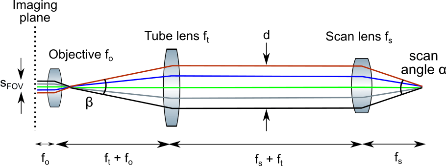
The deflection angle range of the beam, α, is de-magnified by the scan lens/tube lens system to the smaller angle β and then propagates to the objective. The top-bottom spread of the scanned beams on the left indicates the size of the FOV. Using simple trigonometry based on the angle and the distances of lenses to their focal point, one can state (but see also Fabian’s comment below the blog post):

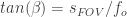
From which one can derive the expected size of the FOV:

Interestingly, the FOV size depends linearly on the ratio f_s/f_t. As we have seen above, the beam diameter at the back aperture of the objective depends linearly on f_t/f_s, the inverse. This results in a trade-off, such that, when you try overfill the back aperture by increasing f_t/f_s, you will automatically decrease the maximal FOV size. It is therefore important to know beforehand what is more important, high NA (and therefore resolution) or a large FOV size. This is not only but to some extent already determined by the choice of scan lens and tube lens.

To give some real numbers, the deflection angle of a typical resonant scanner is 26°. Let’s say we have f_t/f_s=4. The “effective focal length” of the objective is often not obvious nor indicated. As a rule of thumb, the magnification (e.g., 16x from Nikon) together with the appropriate tube lens (e.g., 200 mm) can be used to compute the focal length as 200 mm/16 = 12.5 mm. – Where does the 200 mm come from? This is a value that is company-specific. Most companies use 200 mm as this standard tube lens focal length, while for example Olympus uses 180 mm as default. (As a side-effect, a 20x objective from Olympus has a shorter focal length than a 20x objective from Nikon.)

Together, we have f_o=12.5 mm, α=26°, f_t/f_s=4, arriving at s_FOV=1.5 mm as an estimate for the maximally achievable FOV using these components.

As another side note, when you look up the maximal scan angles of a scanner, there is often confusion between “mechanical” and “optical” scan angle. When a scanner moves mechanically over 10°, the beam will be optically deflected by twice the amount, 20°. For FOV calculations, the optical scan angle should be used, of course.

(3) How to compute the axial focus shift using a remotely positioned tunable lens

The final third example for gemetrical optics is a bit more involved, but it might be interesting also for less ambitious microscope tinkerers to get the gist of it.

I few weeks ago, together with PhD student Gwen Schoenfeld in the lab of Fritjof Helmchen, I wanted to re-design a two-photon microscope in order to enable remote focusing using an electro-tunable lens. Here’s the basic microscope “design” that I started with:

As you can see, the objective, scan lens and tube lens are as simple as in the previous examples. Behind the scan lens (f_s), there is only a slow galvo scanner (for the y-axis), while the fast resonant scanner (for the x-axis) is behind a 1.5:1 relay. There are two ideas behind this “relay” configuration. First, a relay between the two scan mirrors makes it possible to position them more precisely at the focus of the scan lenses (there exist also some more advanced relay systems, but this is a science by itself). Second, the relay system here is magnifying and enlarges the beam size from 5 mm (at the resonant scanner) to 7.5 mm (at the slow galvo scanner). In the end, this results in a smaller FOV size for the x-axis but in a larger beam size at the back of the objective and therefore better resolution.

To insert a remote tunable lens into this system, we had to do this in an optically conjugate plane of the back focal plane. This required the addition of yet another relay. This time, we chose a de-magnifying relay system. The tunable lens had a larger free aperture than the resonant scanner, so it made sense to use the full aperture. Also, as you will see below, this de-magnifying relay system considerably increases the resulting z-scanning range using the tunable lens. For the tunable lens itself, we chose a tunable lens together with a negative offset lens, resulting in a default behavior of the lens as if it did not exist (at least to a first approximation).

Now, before choosing the parts, I wanted to know which z-scanning range would be expected for a given combination of parts. My idea, although there might be simpler ways to get the answer, was to compute the complex beam parameter of the laser beam after passing through the entire lens system. The beam waist and therefore the focus can then be computed as the point where the real part of the beam parameter is zero (check out the Wikipedia article for more details).

To calculate the complex beam diameter after passing through the system, I used geometrical optics. More precisely, ABCD optics. ABCD optics is a formalism to use geometrical optics using 2×2 matrices. A lens or a certain amount of free propagation space are represented as simple matrices, and the beam propagation (distance from center line and angle) is then computed by multiplying all the matrices. For the system above, this means the multiplication of 16 matrices, which is not difficult but takes very long. The perfect tool for that is Wolfram’s Mathematica, which is not free but can be tested as a free trial for 30 days per e-mail address. All the details of this calculation are in a Mathematica Notebook uploaded to Github.

Briefly, the result of this rather lengthy mathematical calculation is a simple result, with the main actors being the axial z-shift in the sample (z) and the effective focal length of the tunable lens (f_ETL):

Using this formula and a set of candidate lenses, it is then possible to compute the z-scanning range:

Here, the blue trace is using the formula above. For the red trace, I displaced the ETL slightly from the conjugate position, making the transfer function more linear but the z-range also smaller, and showing the power and flexibility of the ABCD approach using Mathematica.

Of course, this calculation does not give the resolution for any of these configurations. To compute actual resolution of an optical system, you will have to work with real (not perfect) lenses, using ZEMAX or a similar software that can import and simulate lens data from e.g. Thorlabs. But it is a nice playground to develop an intuition. For example, from the equation it is clear that the z-range depends on the magnification of the relay lenses quadratically, not linearly. Also, the objective focal length enters this equation with the power of the square. Therefore, if you have such a remote scanning system where a 16x objective results in 200 μm of z-range, switching to a 40x objective will reduce the z-range to only 32 μm!

This third example for the use of geometrical optics goes a bit deeper, and the complex beam parameter is, to be honest, not really geometrical optics but rather Gaussian optics (which can however use the power of geometrical ABCD optics, for complicated reasons).

In 2016, I used these mathematical methods to do some calculations for our 2016 paper on remote z-scanning with a voice coil motor, and it helped me a lot to perform some clean analyses without resorting to ZEMAX.

Apart from that, the calculation of beam size and FOV size are very simple even for beginners and a nice starting point for a better understanding of one’s point scanning microscope.